
Chapter 4. Association Between Networks
Relational data describe the ties between pairs of actors. Just as we might ask whether two attributes are associated (e.g. do men and women differ on test scores?), we might ask whether two relations are associated (e.g. are people who are connected by being in the same work group likely to be connected by a friendship tie?). This chapter introduces analyses that examine association between relational data.
In the last chapter we looked at how the relationships among attributes of nodes in a network can be studied statistically. This is really the same as studying statistical association between variables, observed across cases. The only new issue was how to test hypotheses appropriately in the face of the non-independence of the cases.
In this chapter we take a look at studying association between networks. That is, are the relations of one type among the actors in a network associated with relations of another type? For example, are people who are friends outside of work more likely to go to one another for advice at work? In our example student data (introduced in Chapter 2), we might ask how similar the patterns of acquaintanceship are between the beginning and the end of the class, or whether people who were both in the same work group are more likely to be acquainted with each other.
Studying whether two or more networks are associated is actually quite straightforward. Rather than treating the “case” or node as a unit of observation (or a row in our dataset), we treat a “dyad” of nodes as the unit of observation. A first network is “deconstructed” into all possible pairs of nodes (dyads), and the dyadic relationship is measured for each pair (it may be binary, i.e. present/absent—or valued, i.e. tie strength). The other network of interest is deconstructed in the same way. Then, the association between the two can be calculated. The “sample size” then is always equal to the number of unique pairs of nodes. If the network is directed,

where K is the number of nodes in the network. If the network is symmetric,

The trick to studying associations among networks lies in seeing the relation between each pair of nodes as the object of interest (is a tie present?, how strong is it?). A network is seen as simply a collection of (all possible) dyads. The association between two networks is describing the extent to which the scores of one set of relations correspond to the scores of another set of relations among the same actors.
In studying the relationships among networks, the inferential statistical question is not one of generalizability – after all, we have (in theory) directly observed the entire population of actors, so there is no inference from sample to population. But, there is a question of how likely it is that the association we observe between two or more networks is the result of random, rather than systematic processes. So, again, the method of generating standard errors by permutation of the existing data is a useful tool.
Let’s take a look at a few simple examples of the association and partial association among networks using tools from the UCINET toolkit.
Two networks are associated, co-vary, or are correlated to the extent that the patterns of dyadic relations in one correspond to the pattern of dyadic relations in the other. The relation between the actors in a dyad can be measured as either present/absent, or as a matter of degree. Let’s start with categorical relations, which are studied by way of cross-tabulation, then turn to continuous relations, which are studied by way of correlation.
4.2.1 Categorical RelationsSuppose that we want to know whether there is an association between two categorical relations. This somewhat new idea is far easier to grasp with examples. Here’s an obvious hypothesis about the association between two categorical relations: students who were assigned to the same groups to work on their term papers are more likely to report that they are acquainted by the end of the course than students who were not in the same workgroup.
One relation of interest is whether each dyad was in the same work group or not. In Chapter 2, we created an actor-by-actor (i.e. 75 x 75) binary, symmetric matrix using Data>Partition to sets followed by Data>Affiliations (2-mode to 1-mode) and saved the dyadic data as “Same_work_groupRows”. Notice that the unit of analysis is the dyad, and the dyad is characterized as being in the same group (coded 1) or not (coded 0).
The other relation of interest is whether the members of the dyad are acquainted at the time of the last data collection (wave 4). This matrix is the asymmetric actor-by-actor acquaintanceship data. These data are also measured at the binary level.
We can measure the strength of association between being in the same work group and being acquainted, and test significance, using Tools>Testing Hypotheses>Dyadic (QAP)>QAP Relational CrossTabs. The dialog is shown in figure 4.1.
Figure 4.1. UCINET Dialog for Acquaintanceship at End of Course and Same Work Group Crosstab
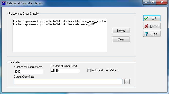
In the dialog, we used the browsing tool to locate each of the two relational (dyadic) matrices. The number of permutations and random number seed defaults are fine (to recreate our output, use the seed above). We elected to not save the output as a new dataset in this case by leaving “Output CrossTab” empty. Figure 4.2 shows the output.
Figure 4.2. UCINET Output for Acquaintanceship at End of Course and Same Work Group Crosstab
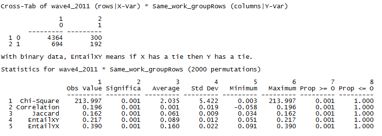
The first panel of the output is the relational cross-tabulation itself. It conveys that there were 4,364 dyads that reported no acquaintanceship tie that were also not in the same workgroup. There were 300 dyads among students in the same workgroup that had no claim of acquaintanceship! Of the students who claimed to be acquainted by the final exam, 192 pairs were in the same work group while 694 pairs were not. Simple ratios demonstrate that the likelihood of being acquainted by the final exam is much higher for those in the same work group: 192/(300+192) = 0.39 vs. 694/(4,364+694) = 0.14.
Given this simple joint count, the second panel of the output calculates various measures of association and tests for significant association using permutation tests. The observed Chi-square value in the cross-tab is 213.997. Across the 2,000 cross-tabs generated from randomly permuted data, the average Chi-square statistic was 2.035, with a standard deviation (standard error) of 5.422. Obviously, our observed chi-square is very unlikely to occur in random data. The strength of the association, however, is not terribly impressive (the correlation is 0.20, for example). Clearly, students placed in the same work group were more likely to claim that they were acquainted than those not in the same workgroups, but it doesn’t look like the group projects made a really big difference in building even weak-tie networks in the class!
As a second brief example, we can look at the stability of reported acquaintanceship over the four waves using Tools>Testing Hypotheses>Dyadic (QAP)>QAP Correlation and choosing all four waves. The resulting Pearson’s correlation matrix is shown as figure 4.3.
Figure 4.3. UCINET Generated Correlations of Acquaintanceship Relations over Four Waves
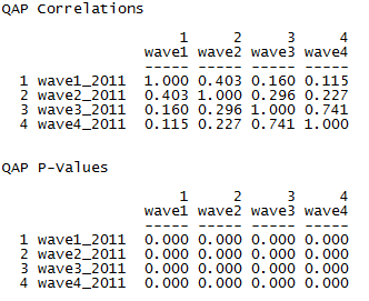
As one would expect, the similarity of acquaintanceship structures declines with the length of period of time between measurements. The largest shift in ties appears to occur between waves two and three. Waves one and two are most highly correlated with one another, and the same is true for waves three and four.
4.2.2 Valued RelationsIn many cases the relation between the members of a dyad is measured as a quantity, or “valued” relation. Valued relations often indicate the strength of a tie, or some similarity between the two actors (perhaps their nearness or closeness in geographical or network space), or the probability that a tie is present. The natural approach to seeing if two networks of valued relations are associated is to compute the correlation between the tie strengths in one relation with the corresponding tie strengths in the other relation.
Two actors might be expected to be more similar (closer), or be more likely to form social ties if they are frequently co-present in social contexts. That is, actors who have the same pattern of affiliation might be said to have a tie. Using data on which classes each student attended, we used the Data>Affiliations (2-mode to 1-mode) tool to create an actor-by-actor matrix of the number of times (potentially 0 to 11) each pair of students had attended the same classes. Dyads with higher values indicate a more similar attendance pattern for the students in the dyad. The same procedure discussed in Chapter 2 (see the dialog in Figure 2.13) can be used to generate this dyadic data.
Let’s say we’re interested in testing the idea that students who attend the same classes are likely to have similar patterns of exam performance. So, again using the attribute data file, we also can calculate how similar the grades of each pair of students were by using the Data>Affiliations (2-mode to 1-mode) tool to create the correlation between students based on the three exam scores (check the box for “Correlation” in the “Affiliations: Convert 2-mode to 1-mode data” dialog). That is, two students are similar, or have a “strong tie” if there is high correlation between scores across the three tests.
Figure 4.4 shows the dialog for calculating the QAP correlation between the similarity in attendance matrix and the correlation of tests matrix. (Tools>Testing Hypotheses>Dyadic (QAP)>QAP Correlation). Our research hypothesis is that students who have similar patterns of class attendance are likely to have similar patterns of grades.
Figure 4.4. UCINET Dialog for Correlation between Two Networks
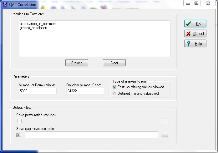
The dialog simply asks that the two (or more) dyadic matrices be identified, and allows control over the permutations and saving the results, which are shown in figure 4.5.
Figure 4.5. Dyadic Correlation of Similarities of Class Attendance and Similarity of Exam Grades
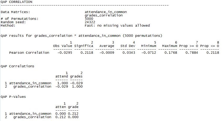
Such a clever hypothesis – and such a disappointing result! We see that there is a non-significant, but negative, correlation between similarity of attendance profiles and similarity of exam grades (r = -0.0295, p = 0.2118, two-tail). Across the 5000 random permutations, the average observed correlation was -0.0009, with a standard deviation (standard error) of 0.03243. The amount of overlap that two students had in the classes they attended appears to have nothing to do with achieving similar results on exams. Note, again, that both of these variables are relational or dyadic, in that they describe the relation between two actors and not the attributes of the individual actors.
Cross-tabs and correlations are quite adequate for studying many interesting questions about dyadic association. But, if we can treat one relation as dependent and the other(s) as independent, we can apply linear modeling to do prediction and partial association as well.
4.3.1 Binary RelationsIf the outcome relation is binary, a natural choice for prediction is binary logistic regression.
Let’s re-visit the question of whether being placed in the same work group is associated with being acquainted by the end of the course. The dependent outcome is the binary, asymmetric, matrix of each student nominating others as acquaintances. The independent dyadic variable is being in the same work group, or not. Figure 4.6 shows the dialog of UCINET’s Tools>Testing Hypotheses> Dyadic (QAP)>LR-QAP Logistic Regression (beta).
Figure 4.6. UCINET Dialog for QAP Logistic Regression of Wave 4 Acquaintanceship by Same Workgroup
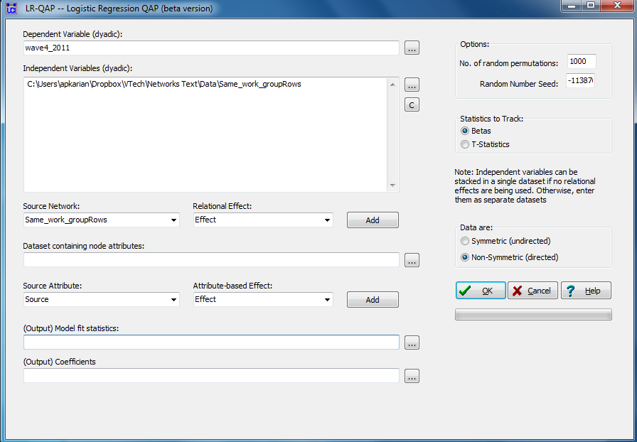
This is a very complicated looking dialog for such a simple question! The reason is that there is much more in this tool than we will be using right now. A bit later on, we will look at a more complex approach to modeling and prediction of networks – exponential random graph (ERG) modeling. The dependent relation or network is our non-symmetric (see the selection of symmetric/non-symmetric on the lower right in the dialog) wave 4 acquaintanceships. Our single “independent” network or dyadic variable is the matrix of “in the same work group.” At present, we won’t use the “relational effect” or “attribute-based effect” parts of this tool. Note that the regression output can be saved with the output file boxes at the bottom of the dialog.
Figure 4.7 shows the output of our logistic regression model. By the way, ERG models with permutation can take a rather long time to run. So, be (reasonably) patient.
Figure 4.7. UCINET Output for QAP Logistic Regression of Wave 4 Acquaintanceship by Same Work Group
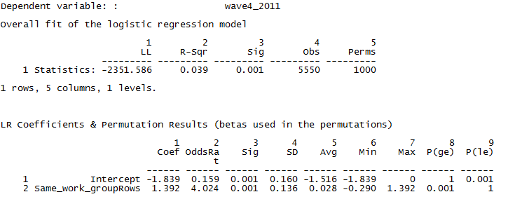
The output first reports the overall goodness-of-fit of the model. The log-likelihood is given, along with the likelihood-based pseudo-R square statistic. Note that the N is 5550, or the number of directed pairs formed by 75 nodes. We can conclude that being in the same work group does affect the log-odds of naming another member as an acquaintance (the coefficient is significant; p = 0.001), but that this tendency explains a tiny proportion of the variation in likelihood of being acquainted (pseudo-R square = 0.039).
The regression coefficients show the additive effects on log odds (Coef), or multiplicative effects on odds (OddsRat) of naming alter as an acquaintance. The simple summary here is that being in the same work group as alter multiplies the odds that ego will name them as an acquaintance by about 4 times (4.024). The average regression coefficient in 10,000 random permutations of the data was 0.028, and the standard error was 0.136.
Since we are now working in the generalized linear modeling framework, there is no difficulty in adding additional variables as partial explanations or control variables. In figure 4.8, we’ve added whether an acquaintanceship was reported at wave 1, wave 2, or wave 3, as well as having similar attendance records and similar exam grades as additional predictors of acquaintanceship at the end of the course.
Figure 4.8. UCINET Output for QAP Logistic Regression of Wave 4 Acquaintanceship on Multiple Predictors
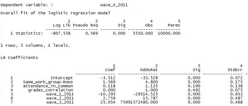
The overall fit of the model is now very much better. However, most of the improvement is due to including the presence of ties earlier in the term as predictors of ties at the end of the term. Note that, while significant, the autoregression of current social ties on earlier ones has substantial collinearity and produces some very unstable results (UCINET’s routines do not include VIF or other collinearity statistics). Our “test” variables can be interpreted as attempting to predict the presence or absence of ties that would not have been expected based on the trend in the development of ego’s network. Having similar grades has no discernible partial effects at all. Having a similar attendance profile is very slightly (but not significantly) partially associated with being acquainted. But, the positive effect of being in the same work group is strengthened somewhat by controlling for the other variables.
The UCINET tool for predicting a binary dyadic dependent variable is quite easy to use for simple models. The prediction of a binary dyadic relation from any combination of independent variables can also be approached with specialized software that takes graph structure into account (exponential random graph models), or multi-level generalized linear models. We’ll return to these more general tools in later chapters. In the example above (Figure 4.8), earlier observations were used as predictors of later relations; the data are actually panel data. Specialized models for studying change in dyadic relational variables are also available (e.g. Siena).
4.3.2 Valued RelationsThe same logic and approaches can be applied where the outcome dyadic variable is an interval-ratio level measure of dyadic tie-strength. Figure 4.9 shows the dialog of the UCINET dyadic regression tool (Tools>Testing Hypotheses>Dyadic (QAP)>MR QAP Linear Regression>Original (Y Permutation) method).
In this example, we are attempting to predict the correlation between the exam grades of the two members of each dyad based on the similarity of their attendance patterns.
Figure 4.9. UCINET Dialog for QAP Regression Predicting Grade Similarity by Common Attendance

The regression dialog is simpler, and has a slightly different appearance. The dependent network is selected in the first box. One or more independent dyadic variables (networks) are selected in the second. Figure 4.10 shows the resulting output.
Figure 4.10. UCINET Output of Grade Similarity by Common Attendance

The results are consistent with those found in Figure 4.5. The model fit panel tells us that any association between similar grades and similar attendance could easily be explained by random processes (p = 0.388). We really should not bother to look at the regression slope. If we did, we would note that the tendency in the data (a standardized slope of -0.03) contradicts our research hypothesis.
However, there may be other factors suppressing the true relationship between attendance similarity and grade correlation so let’s add some control variables. Figure 4.11 shows the multiple regression output of predicting similarity of grades from common attendance patterns, while controlling for being in the same work group and the presence of acquaintanceship at any point during the academic term.
Figure 4.11. UCINET Output of Grade Similarity by Multiple Predictors
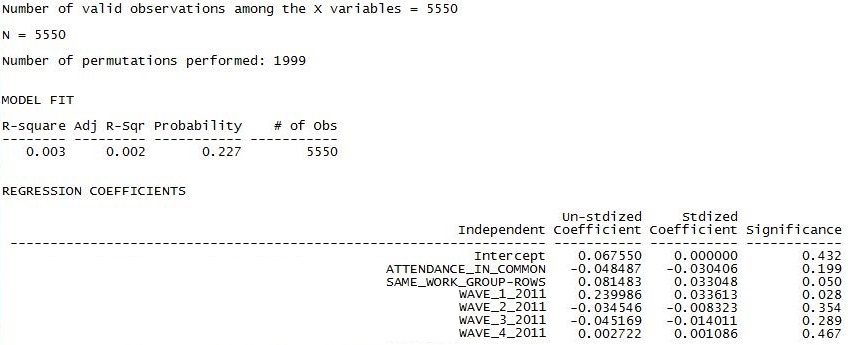
The results are not impressive. Looking at the overall goodness of fit, we should conclude that the similarity of the grades between ego and alter is essentially random with respect to these predictors. Poking into the partial slopes (which we really shouldn’t do), we see that direct acquaintanceship ties only seem to matter at the beginning of the quarter – probably reflecting friendship relationships that existed before starting the class. Being in the same work-group also appears to be associated with having more similar grades. Just as in the bivariate model, attending the same classes is not associated with getting similar grades.
In this short chapter we’ve considered the question of how to study whether the pattern of one set of ties among a given set of actors is similar to the pattern of another set of ties among the same actors. That is, the association of two (or more) networks.
The approach that we’ve looked at here examines each network as a collection of the relations of all possible pairs (dyads) in the network. This treats the dyad as the unit of observation, and the relation between them as the variable to be studied. Approached this way, the conventional tools of tables, correlation, and regression can all be applied to the association between networks.
The inferential statistical question in examining the relationships among two or more networks is not really one of generalization to a population. Rather, it is whether the observed degree of correspondence or similarity between two relations among the actors in a network could have happened by random processes. So, for testing hypotheses about the relations among networks, the permutation method for estimating standard errors is ideal.
The tools that we’ve looked at in this chapter are actually quite simple. But, they can be useful for many interesting questions. Later on, we’ll see more complex approaches (exponential random graphs models and multi-level models) to examining entire networks as dependent variables that allow for much more complex and interesting hypotheses.
We’ve now looked at how to examine the association between two or more attributes when they are observed on actors embedded in a network (Chapter 3). We’ve also looked at how to examine the association among two or more networks (this chapter).
Logically, this raises the question of how one might study the association between attributes and networks – i.e. the association between nodal and dyadic relational variables. Read on!