Back to Table of Contents

Chapter 3. Association Between Attributes in Network Data

Having looked a bit at how attribute and relational data are structured, we are ready to start doing some statistics. In this chapter we will look at a type of analysis that is very familiar: studying the association between two variables. In SNA, this is commonly referred to as studying the association between two attributes of the actors in a network.

3.1 Association Between Attributes in Network Data

3.2 Univariate Statistics for Attributes

3.3 Association Between the Attributes of Embedded Nodes


3.3.1 Comparing Two Groups

3.3.2 Comparing Multiple Groups

3.3.3 Continuous Association


3.4 Partial Association and Prediction of Attributes by Attributes

3.4.1 Multiple Regression

3.4.2 Generalized Linear Models


3.5 Summary

3.6 References

The notion of studying the association between two variables (while possibly controlling for others) is the bread-and-butter of conventional statistical analysis.  So, it shouldn’t be surprising that social network analysts are often interested in the association between two (or more) attributes observed across the actors in a social network.  With our example data that was introduced in the last chapter, we could test the hypothesis that women were more likely to have higher participation scores in their research groups than men, for example.  We would like to know how strong such a tendency is in our observations (that is, measure the strength of the association); and, we would like to test the null hypothesis that the observed association was the result of a random process.

In the last chapter, we noted that SNA also thinks about how actors are embedded in networks as attributes of the actors – operating to provide opportunities and imposing constraints on their attitudes and behaviors.  For example, individual students who are in highly central positions in the classroom network might be more likely to have higher grades.  In this case, the centrality of the student in the network is being thought of as an attribute of the individual.  How attributes of nodes are related to their positions in the network are key questions asked in SNA (e.g. are men more likely to have higher network centrality than women?).

Studying the association and partial association among attributes of actors in a network is done with exactly the same tools as are used in studying association among variables.  Cross-tabulations, tests for differences of means of two or more groups, correlation and regression can all be applied to describe the strength and form of association between the attributes of actors in a network.  The descriptive statistics used for association with the attributes of nodes are exactly the same as the descriptive statistics used to describe the association between variables across cases.

But, when we turn to the question of inference and hypothesis testing, we come to a new issue.  The formulae that are used to calculate standard errors and test statistics for variation of variables across cases most commonly assume that the cases are independent replications – and often, randomly drawn from an infinite population.  SNA data, most commonly, are not samples but populations.  And, SNA data are, by definition, not independent replications.  It is precisely the non-independence of the cases that is of central interest to SNA!  When we measure the association between two traits or attributes of actors who are connected to one another by social ties, it is quite likely that the social ties might have been created, at least in part, as a result of the attributes of the actors.

In testing hypotheses, the logic is to compare some statistic or parameter (for example, a measure of association or partial association) to how much we would expect that statistic to vary from one set of observations to another just by chance (the standard error).  The standard error, or sampling variability, or reliability is a statistic often calculated using standard formulae that assume independence.  With social network data, standard errors need to be computed differently.  Conventional standard errors will be biased – they may be too big (leading us to incorrectly reject a true hypothesis) or too small (leading us to incorrectly accept a false hypothesis).

Estimating standard errors for non-independent observations is a common problem, and has many solutions.  Probably the best known and most widely used approaches are the jack-knife, bootstrap, and permutation methods (Efron, 1981).  For SNA, the logic of permutation is quite appealing, and is widely used in UCINET.

The basic idea of the permutation trials method is to take the existing data on the attributes of the nodes and randomly re-assign the scores on one attribute.  The parameter we’re interested in (for example, the Pearson correlation between student’s attendance and test scores) is then measured in the permuted dataset, where the relationship between the two attributes is the result of a random trial.  This procedure is repeated a number of times (say 1,000 or 10,000), and the distribution of the statistic across the random trials is calculated.  We then compare the observed statistic against this random distribution to find out how frequently the statistic would be observed in random trials.  It is a simple (if computationally a bit demanding) approach that preserves the observed distributions of both attributes – whatever they might happen to be – and requires no assumptions about sampling.

Usually the most interesting research questions call for examining association, partial association, and prediction.  But, it is always a good idea to first examine each of the variables, one at a time.  Since attribute data are stored as conventional rectangular data (cases by variables), any statistical package can be used to examine the distributions of the variables.

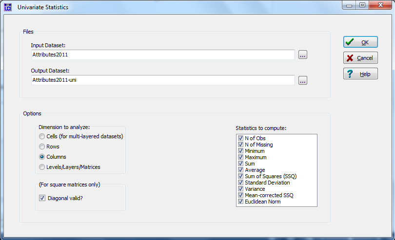
For quantitative attributes, UCINET’s Tools>Univariate Statistics will do the trick.  Let’s look at our student data.  The dialog is shown as figure 3.1.

Figure 3.1. UCINET Dialog for Attribute Univariate Statistics

The dialog is very simple. We select the name of our attribute file, and specify “columns” to calculate the statistics on the distribution of the attributes across cases. The matrix is not node-by-node, so the question about the diagonal doesn’t apply. The output can be saved as a UCINET data file (also rectangular, variables by statistics), and/or cut-and-pasted from the output log. A portion of the output is shown in figure 3.2.

Figure 3.2. Portion of UCINET Output for Attribute Univariate Statistics

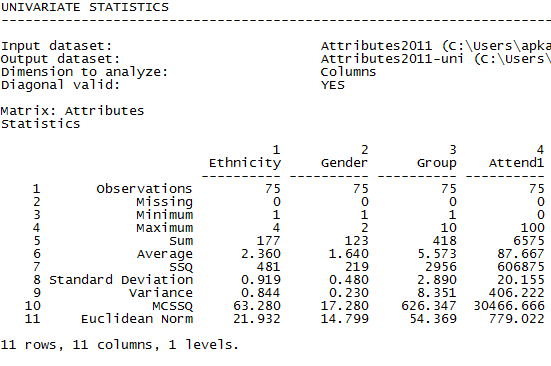
The report gives all the conventional basic descriptive statistics, N, minimum and maximum, as well as some additional measures of variation. UCINET doesn’t compute skewness and kurtosis. For our categorical variables of gender, ethnicity, and work group, moments are not particularly helpful. However, for continuous variables like Attend1 (percentage of in-class quizzes completed in weeks 1-3; up to the first exam), these statistics are useful.

A frequencies table would be nice, and UCINET does provide one – though it is not ideal. Figure 3.3 shows the dialog for Tools>Frequencies.

Figure 3.3. UCINET Dialog for Attribute Frequencies

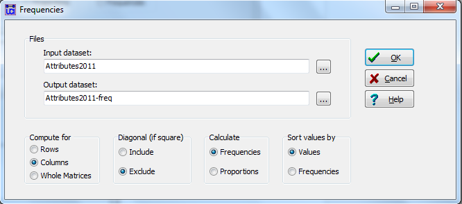
Figure 3.4. Partial UCINET Output for Attribute Frequencies

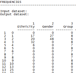
Figure 3.4 shows a portion of the output.  We can still see that women outnumber men about 2 to 1 (48 to 27), that 17 students identified as White, 20 as Hispanic, 32 as Asian, and 6 as African American in the class.

Let’s now turn to bi-variate association of nodal attributes.

There are many different approaches to examining association or covariation between two variables, depending on the levels of measurement of the variables and the purposes of the analysis.  Some of the most common approaches are to build cross-tabulations (for two categorical attributes), compare two or multiple group means (for one categorical and one continuous attribute), or use correlation and regression to examine two continuous attributes.  UCINET does not have a tool for cross-tabulations and permutation tests for categorical association.  For problems of that type, statistical software that will run boot-strapping, jackknife, or permutation should be used.  In Stata, for example, one can embed a regular call for a tabular analysis within permutation trials with syntax such as:

Permute Y  “text of the cross-tabulation command, options”  name-of-statistic desired , reps(n)

The permute command tells Stata to randomly permute the values of the variable Y (i.e. one of the variables in your cross-tab).  The text of the tables command is then embedded in quotes (e.g. “tabulate Y X, chi2”).  Following the crosstab command, a report on the values of one or more saved statistics is requested (e.g. perhaps chi-squared; saved in local memory as “r(chi2)” by the “tabulate” command), and the number of desired random replications is specified.

To test hypotheses about the association between a binary attribute (e.g. gender, in our data set) and a continuous one (e.g. exam scores), we can calculate a standard two-group t-test.  In UCINET, the dialog can be located at:  Tools>Testing hypotheses>Node level>T-test.

Let’s look at two examples.  We first look at whether there are gender differences (a fixed binary attribute) in mean final exam scores (a continuous attribute).  Following conventional wisdom, our research hypothesis is one-tailed:  we expect that the women’s mean will be higher than the men’s.  Figure 3.5 shows the dialog.

Figure 3.5. UCINET Dialog for a Two-group T-Test

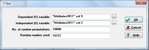
Only two things to note here:  First, you must know which column your variable is located in (final exam score happens to be column 9 in the attribute dataset, and gender happens to be column 2).  UCINET will suggest column 1 by default, and you can simply edit it.  Second, you can select the number of random permutations for significance tests.  The default is 10,000, which is more than adequate for most purposes.  Note the “random number seed.”  You may wish to generate the same permuted distribution for multiple tests.  This can be done by noting, and then specifying that the same seed be used to start the pseudo-random number generator.  Figure 3.6 shows the output (try replicating Figure 3.6 using the seed 16721).

Figure 3.6. UCINET Output for Testing Gender Differences in Final Exam Scores

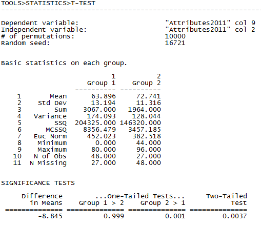
Here, we need to note that UCINET takes the value of the categorical variable (gender) from the first case and calls that “Group 1”.  So in this output, Group 1 happens to be women (coded 2 on the variable) due to the arbitrary fact that the first case in the dataset is a woman.  This can be confusing, so the user should always check the attributes of the first node (or the “N” value if they differ; for example, we know the N for women is 48 from figure 3.4, therefore Group 1 in Figure 3.6 is women) to make sure they know which group is which.  The output shows the descriptive statistics for the two groups.  Women have a mean test score of about 64, while the men’s average is about 73, in contradiction to our research hypothesis.  The variation within each group, however, is substantial, and there are considerably more women than men.  In the significance tests section, we see the difference in means and three probability levels based on the standard error of the difference between means generated from the permutation trials.  The interpretation is as follows: in over 99.9% of random networks with the same numbers of men and women and the same univariate distribution of test scores, the mean of group 1 (women) is NOT higher than the mean of group 2 (men).  In more than 99.9% of the trials, the mean of group 2 (men) is higher than group 1 (women).  In about one third of 1% of the permutation trials, the difference in means observed between groups is less than the average difference observed in random trials.

Figure 3.7. Stata Test of Gender Difference in Final Exam Scores with Conventional Standard Errors

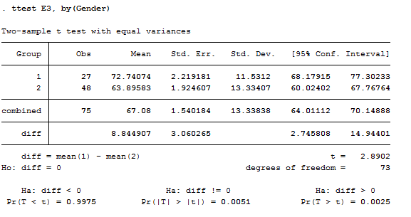
Figure 3.7 shows the same problem, but tested in Stata using conventional standard errors.  In this case, we see that the statistical significance (p level) of the test of the difference between the two group’s means is stronger using the standard error estimated by permutation trials than using the classical formula (the two-tail p-level for the permutation test is 0.0037, the two-tail p-level using the classical formula is 0.0051).  Standard errors and significance results may be either stronger or weaker using the permutation method than the classical formulas.

In the next example, we ask whether the average in-degree of women (that is, the number of others who say they are acquainted with them) is different from the average in-degree of men at the time of the final exam.  We can calculate the in-degree of each node using Network>Centrality and Power>Degree in UCINET.

Figure 3.8. UCINET Dialog for Generating Degree Data

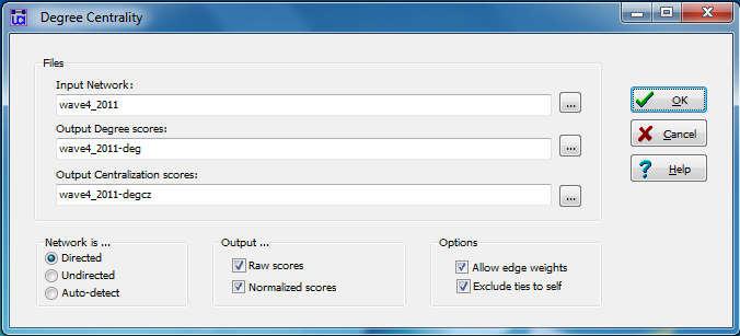
Here, we’ve chosen the Wave 4 relational data, specified that it’s directed, and UCINET saves measures of degree and centrality in separate files.  We can use the Data>Join>Join Columns procedure to append the degree attributes generated in the file “wave4_2011-deg” to our “Attributes2011” file and create a new dataset called “Attributes2011_degW4” (the Join procedure was discussed in greater detail in Chapter 2).  When running a t-test for differences in in-degree between men and women, the dialog is the same as in Figure 3.5, except that we have selected different variables (in-degree will be column 13 in the new joined dataset).

The reason for a second example of a simple two-group t-test is to point out that attributes can be measures of how individuals are embedded in social networks.  The in-degree of a node describes dyadic relations (someone else said they were acquainted with ego).  But, the extent to which a node has dyadic ties is an attribute of the node itself.  The output from the t-test is shown in Figure 3.9.

Figure 3.9. UCINET Difference in In-degree Between Men and Women Students (Wave 4)

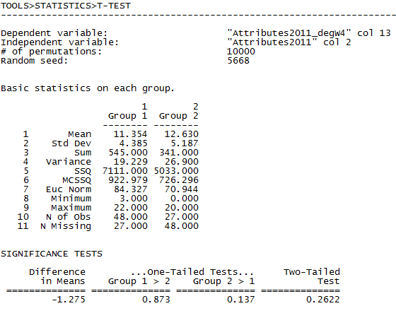
We see that the mean in-degree of men students (group 2) at the end of the course was a bit higher than that of women.  Using the standard errors of the difference in means generated by permutation tests, we see that a difference this large occurs relatively frequently in randomly permuted networks (26% of the random networks).  Therefore, we do not find support for the notion that the difference in the average in-degree of men and women students is not due to random processes.

If one of the attributes is categorical with more than two categories, and the other attribute is continuous, a common approach to testing hypotheses is one-way ANOVA (in UCINET: Tools>Testing Hypotheses>Node Level>ANOVA).  Let’s see if there are any significant differences between the mean final exam scores of students classified by ethnicity.  The dialog is in figure 3.10, and the output is in figure 3.11.

Figure 3.10. UCINET Final Exam Score Means by Ethnicity Dialog

Figure 3.11. UCINET Final Exam Score Means by Ethnicity Output

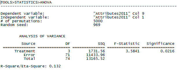
UCINET’s output is minimal, providing the standard ANOVA table, F-test statistic, and significance.  Eta-square is also shown.  We conclude that to 95% confidence, there is at least one difference between group means that is not expected to occur very frequently in random permutations of the data.  And, group mean differences account for 13.2% of the observed variation in individual’s final exam scores.  That is, the differences among mean final exam scores by ethnic identity probably are not due to random variation (though there may very well be spurious factors at work here).

Let’s see whether there are differences by ethnic identity in the extent to which individuals are named by others as acquaintances.

Figure 3.12. UCINET Node In-degree by Ethnicity Dialog

Figure 3.13. UCINET Node In-degree by Ethnicity Output

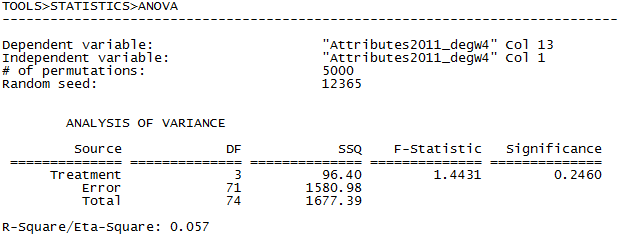
In the classroom data, it looks like there are no reliable differences due to ethnicity in the extent to which students are likely to be known by others in the class.

Where one or both attributes are measured at the ordinal level, the standard approach is to calculate measures of association (e.g. gamma).  UCINET doesn’t have built in tools for calculating hypothesis tests for grouped-ordinal variables.  Statistical software packages that allow calculation of estimated standard errors with re-sampling or permutation should be used.

For problems where both attributes are interval-ratio, or can reasonably be treated as such, UCINET has built-in tools for using linear regression (Tools>Testing hypotheses>Regression).

Let’s examine whether students who name more others as acquaintances than average (out-degree) are, themselves, more frequently cited by others (in-degree).  Again, variables that describe how individuals are embedded in the network (in-degree, out-degree) are being treated as attributes of the individuals.  Obviously, standard significance tests don’t apply, as the nodes generating the degree counts are the same individuals.

Figure 3.14. UCINET In-degree and Out-degree Regression Dialog

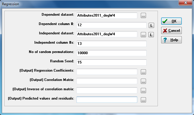
In the dialog, note that the dependent and independent variable can be taken from different datasets (one might be a file of attributes, the other a file of results of calculating network statistics like degree or centrality).  All of the important regression output can be saved in output data files for further processing.  We’ve left the boxes blank here so as not to save the output as new datasets.

Figure 3.15. Portion of UCINET In-degree and Out-degree Linear Regression Output

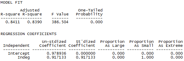
From the output, we see that there is a strong positive association on out-degree with in-degree (+0.917).  The variance explained in in-degree by out-degree is considerable (0.841).  Each additional person named by ego as an acquaintance is associated with an increase of 0.917 others naming ego as an acquaintance.  A two-tailed p-level for the coefficient is reported as < 0.001 (under “Proportion As Extreme”).

Let’s run the same problem in Stata, using both the conventional standard errors and permutation trials to test the slope coefficient.

Figure 3.16. Stata Regression Output with and without Permutation Trials

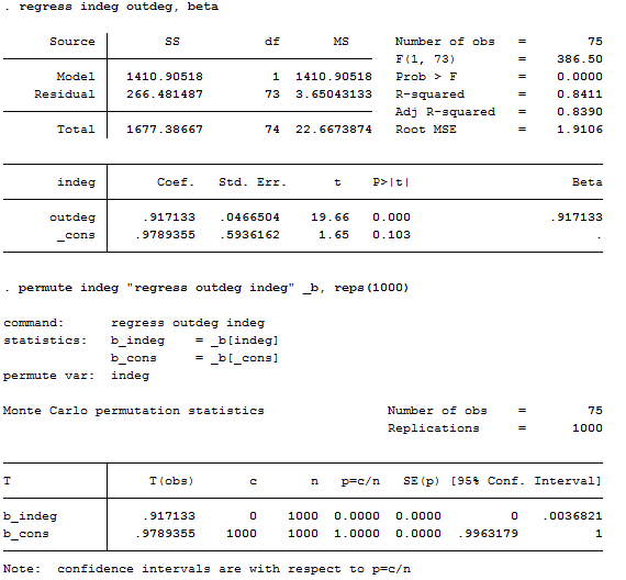
Stata reproduces the regression coefficients and R² statistics.  Notice that the conventional standard error approach and permutation trial approach produce identical results for this example.

While many useful hypotheses can be addressed with simple bi-variate association, most of our work uses variations of the generalized linear model to implement statistical control via partialling.  UCINET has basic tools for multiple linear regression with permutation tests, and this is a nice tool when the attribute we are interested in predicting is measured at the interval-ratio level.  Because the significance tests are based on permutations, we do not need to assume the normality of the distribution of residuals.

As an example, let’s extend our efforts to predict which students were more likely to perform well on the final exam (E3).  Here’s an example of the UCINET dialog for regression that specifies multiple independent variables.

Figure 3.17. UCINET Multiple Regression Dialog

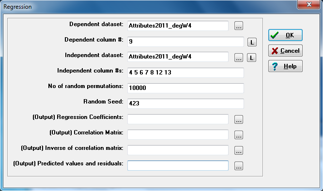
The dependent variable is selected as the desired column in one attribute data set.  The independent variables are selected by column numbers from the same data set, or a single different data set.  The number of permutations and seed can be selected, and all of the basic regression output components can be saved for further processing or reporting.  The output is presented in Figure 3.18.

Figure 3.18. Portion of UCINET Multiple Regression Output

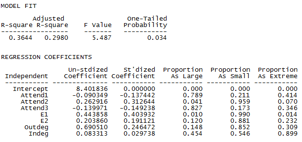
Scores on the final exam (E3) turn out to be moderately predictable, with a significant F-value and adjusted R-square of about 0.3.  Score on the first midterm (E1) has the largest significant effect on the final exam score, but attendance during the middle of the term is also a significant predictor (p < 0.05, one-tail).  Score on the second midterm (E2) also has a positive effect on E3, but only in 88% of random trials which cannot be considered significant based on typical social science statistical standards.  Neither measure of embeddedness is strongly related to exam performance, with nodes that are more popular (in-degree) than we would expect for their sociability (out-degree) showing a tendency to perform better, net of other factors.  But again, this effect is not significant to 95%.

Finally, let’s compare the results of the permutation tests to the regular parametric tests, which are shown in Figure 3.19, where they were calculated with Stata.

Figure 3.19. Stata Regression Output

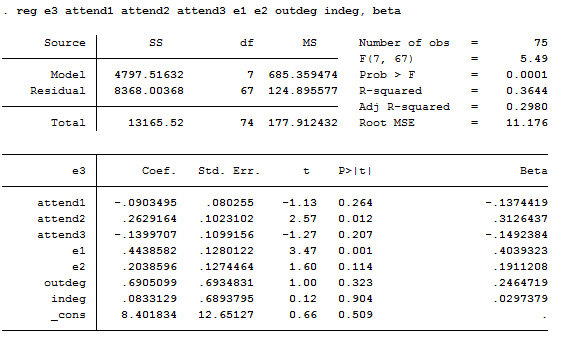
More accurate estimates using permutation trials guard us against committing errors of assuming that effects are systematic, when they might well really be unreliable.

Where attributes of interest are not Gaussian, one should use a statistical package with GLM and appropriate dependent distribution and link functions.  Most scientific statistical software suites include a wide variety of modeling approaches for attributes with varying properties.  Generally, Monte Carlo or permutation trials methods are available to get corrected standard errors and significance tests – though sometimes it requires a bit of work.

Attributes of nodes might sometimes be a count of something.  For example, we might count the number of children that an ego has had and explore whether this is associated with the attributes of ego’s friends.  A Poisson or Negative Binomial model might be used.

Attributes of nodes might be binary (for example, ego is a drug user, or not).  Logistic, probit, or complementary log-log models might be used.

Attributes of nodes might be “multiple choice” outcomes (e.g. ego is working full time, part time, unemployed, or not in the labor force).  Multinomial logits or probits might apply, or ordinal cumulative logits and probits.  See textbooks describing general linear modeling for details (e.g. Hoffman, 2004).

Virtually any hypothesis about the relationships between nodal attributes in SNA data can be studied using the modeling techniques that are used for data based on other observational schemes.  Social network data, though, are usually populations rather than samples.  So, the questions of “generalization” from the sample to the population usually do not arise.  Inferential statistics are necessary, though, as the results in one observation of a network may appear to be systematic, but are really the result of an unusual outcome of a random process.  Permutation approaches (Monte Carlo simulation) provide a natural tool for testing the reliability of results with social network data.

Measures of network position can be used as attributes of individuals (for example, degree, centrality, closure of ego networks, homophily of ego net, proportion of others who have adopted or have some attribute, or the average score of those connected to ego).  Conventional statistics then can be used to include some powerful social influence and embedding information in tests about ego’s attributes, in addition to ego’s fixed individual attributes.  In a later chapter we will look at some other ways of studying how the attributes of those to whom a node is connected might impact the node’s attributes (network influence models are discussed in Chapter 6). 

Conventional approaches to estimating standard errors and hypothesis testing are not appropriate when using social network data, because the “cases” (nodes) are not independent.  But, this turns out to not be much of a problem.  The logic of permutation trials to generate estimates of reliability of parameters fits naturally with SNA.  UCINET adopts this approach for some common tests.  Virtually any hypothesis though, can be tested by using permutation in combination with generalized linear models. 

In this chapter, we’ve discussed how to study the relationship between two (or more) attributes of nodes (or, variables measured on cases).  The unique contribution of SNA, however, lies in treating the relationship or tie between nodes or cases as the thing to be explained and understood.  In the next chapter, we’ll take a look at some approaches to studying the relationships between two or more attributes of relations, or dyads. 

Efron, Bradley. 1981. “Nonparametric Estimates of Standard Error: The Jackknife, the Bootstrap and Other Methods,” Biometrika, 68(3): 589-599.

Hoffman, John. 2004. Generalized Linear Models: An Applied Approach. Pearson.