Chapter 2. Working with Relational Data
In this chapter, we will look at some of the main ways in which the data for SNA are structured for use in statistical analysis. Our examples will use UCINET, which is good for many basic statistical analyses of network data (on fairly small data sets). We will also briefly discuss how network data can be structured for use in multi-level modeling and exponential random graph modeling.
Many of the ideas and the terminology of the statistical analysis of social network data can be a bit difficult when discussed in abstract conceptual terms. However, they become clearer when we apply them to actual data. We will start the chapter by taking a look at the dataset that will be used for most of our examples throughout the text.
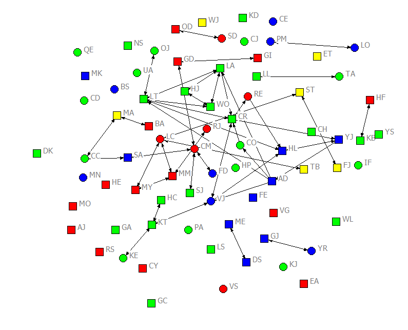
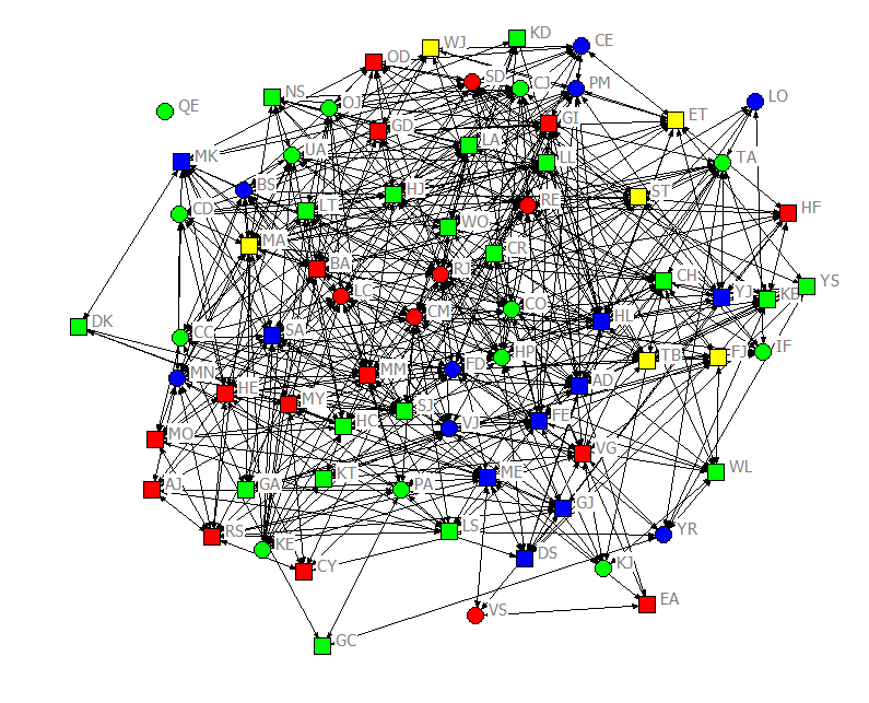
For most of our examples here, we will be using some data about the students in an upper division, undergraduate course in social networks (taught in the fall term of 2011). The data are a population census (not a sample, or set of ego-networks). The students were asked to report about acquaintanceship (i.e. “who in the class do you know well enough to ask a small favor, like borrowing class notes?”), on four occasions over the 11-week class. That is, the design is a panel, rather than a single-cross section, or continuous time set of observations. Information was also collected about some “fixed” attributes (ethnicity, gender), and about some “time varying” attributes (attendance, grades on examinations) that occurred over the term. The acquaintanceship networks for the four waves are shown in figures 2.1 through 2.4, colored by ethnicity (blue = White; red = Hispanic; green = Asian; yellow = African-American), with men shown as circles and women as squares.
Figure 2.1. Acquaintanceship Network for Classroom Data, First Day of Class

Figure 2.2. Acquaintanceship Network for Classroom Data, First Mid-term Exam
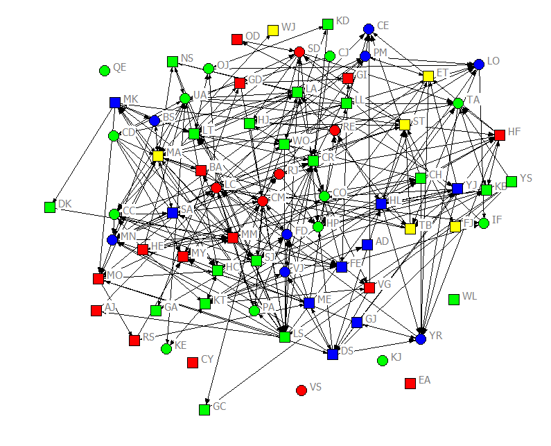
Figure 2.3. Acquaintanceship Network for Classroom Data, Second Mid-term Exam
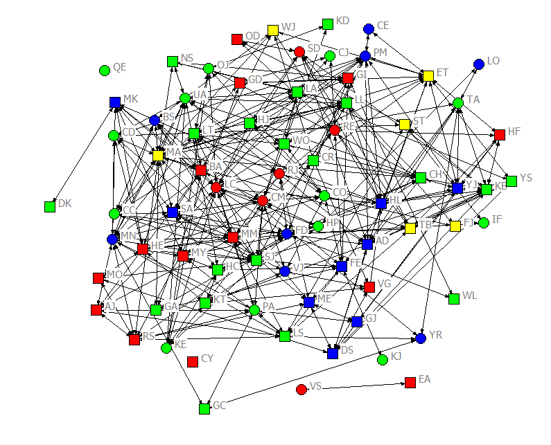
Figure 2.4. Acquaintanceship Network for Classroom Data, Final Exam
More complete details about the classroom data are available on this page. Readers will also be able to download the data there as well in both UCINET and Excel formats. The text was written so that readers can follow the examples by recreating them on their own.
There were seventy-five students in the class. Over the academic term, the density of ties increased quite a lot. On the first day of class, there were 78 unique ties (Figure 2.1). By the first midterm, there were 315 (Figure 2.2). By the second midterm, there were 530 (Figure 2.3). And at the time of the final exam, there were 895 ties (Figure 2.4). Notably, not all students who said that they were acquainted had reciprocated ties. For example, in the center of Figure 2.1, we can see that CO indicated that they knew CR, but CR did not acknowledge CO as an acquaintance. In the same figure, AD claimed to know CO, but CO did not acknowledge knowing AD. Network ties that are not necessarily reciprocated are referred to as “directed” ties. There were more women than men in the class, but reasonable numbers of each gender. The class had considerable ethnic diversity, with more students identifying as Asian than any other group.
SNA analysts use a wide variety of research designs, sampling, and measurement. Design, sampling, and measurement choice all greatly affect how the resulting data need to be analyzed. We can’t hope to be comprehensive in this text. This data set lets us illustrate the kinds of questions and approaches that are most common in current social science work. Understanding the basics with a fairly simple and familiar example is a starting point for analysts with more complicated problems.
Most of the examples in this textbook are done in UCINET, which is why we made the data available in UCINET data files. UCINET data are stored in pairs of files, one with the extension .##h and the other .##d. You can call either one to open the data. The .##d file contains the actual data, and the .##h file contains information on how to call and read the .##d file. You will need to download and store both in the same folder to open a dataset. One set of files used for examples throughout this text is titled attributes2011, which holds the student attribute data. The other four sets of files (wave1_2011 through wave4_2011) contain the acquaintanceship data indicating which students nominated which other students as acquaintances.
What is unfamiliar about the statistical analysis of social network data is its focus on relations between cases as the “unit of analysis,” rather than the more familiar focus on attributes of individuals (which vary across individuals, and are called “variables” outside SNA).
SNA does work with variables, though. It thinks about them as “attributes” of nodes. For example, a conventional, variable oriented analyst might say that “Susan has the score or value of woman on the variable gender.” A social network analyst would say “the node Susan has the attribute woman.”
Sometimes attributes play the role of independent variables used to explain or predict network variables. For example, are women students in our class (“woman” being an attribute of each individual) more likely to be acquainted with other women than they are with men?
Sometimes attributes play the role of dependent variables, predicted by network variables. For example, is a student’s performance on a test (an individual attribute) predictable from the scores on the test of those the student is acquainted with (an observation about dyads)?
Recording data about the attributes of individuals for use in UCINET and other network software is quite familiar. Data are arrayed in the conventional “rectangular” way (cases by variables) or “vector” (cases by a single variable). Figure 2.5 shows a portion of the attributes dataset for the student data. The display is a screen-shot of the dataset viewed through the UCINET Matrix Editor (note: data arrays like this can be created in any software and saved as text files to be imported into UCINET later).
Figure 2.5. Partial View of the Student Attributes Rectangular Data Array in UCINET
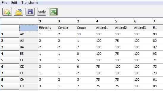
In UCINET, it is best to make sure that each case’s ID is short and a single string, preferably without special characters or spaces. Cases need to be sorted in the same order in the attribute file or files as they are in the relational (dyadic) datasets discussed shortly. It’s good to keep a codebook, as UCINET procedures often ask you for a variable number in the attribute set (e.g. Ethnicity is col. 1, Group is col. 3).
All the standard approaches to coding categorical, ordinal, and interval level variables apply. It is usually best to do most data transformation and elaborate coding outside of UCINET (say in a spreadsheet or statistical package). UCINET does offer some special tools for working with attribute data, however, that we will discuss below. Before turning to these tools, let’s briefly discuss some categories of attribute variables that are used in SNA.
Most specialized social network analysis software systems record information about nodal attributes in the same general way as UCINET. However, each attribute is generally stored in a separate text file (with the cases sorted in the same order across all the files, and varying header information). When relational data is analyzed using mixed-effects generalized linear models, each data line refers to a relation (dyad), and the attributes of the nodes associated with the dyad are coded with each data line.
2.2.1 Fixed and Time-varying AttributesSome attributes that we might be interested in analyzing are ascribed characteristics of individuals that are fixed for each node. For example, in our data set, a student’s gender and ethnicity are treated as static across the four waves. In the statistical analysis of network data, fixed attributes often are used to partition the network (divide it into groups of cases with the same attribute). In mixed-effects modeling, attributes are “level 2” variables (because dyads are the primary unit of analysis – level 1), and dyads are nested in the crossing of two individuals.
Other attributes of individuals may vary over time. In our example, exam score (E1, E2, E3), attendance, term paper score, and term paper team participation all occur at particular points in time. Some might be treated as repeated events or latent growth curves (exam scores or attendance, for example). Time varying covariates may be treated as causes of how a person selects their networks (do students who perform badly on exam 1 create more ties with students who performed better?). Alternatively, time varying covariates might be treated as outcomes of network influence (e.g., does a student’s test score on the second exam depend on the test scores of the others in their network at the time of the first exam?).
All in all, these kinds of variables or attributes are entirely familiar. There is another kind of attribute data used in SNA that might not be quite as obvious.
2.2.2 Network Position as an Individual-level AttributeOne of the key ideas of SNA is that how an individual is “embedded” in the network may affect either their attributes and behavior, or their selection of social relations (making and breaking ties). For example, one important hypothesis is that of “preferential attachment.” This principle says that individuals who have more network ties are more likely to be sought as partners than those who have fewer ties. In this case, the number of ties that an actor has is viewed as a variable or attribute of the actor that affects the probability that they will form more ties.
It is very common for analysts to calculate measures of an individual node’s position in the network and save these as attributes of the node for further analysis. The specific aspects of a node’s position that might be relevant, of course, will vary with the goals of the analysis. A node’s degree, their centrality, the clustering of their ego-network, and the homophily of their ties (the proportion of their ties that are ties to others with the same attribute as themselves) are common things about an individual’s network position that are often treated as nodal attributes in further analysis. While such variables describe a node’s position in a network, the variables are actually an attribute of the node, and can be treated as such.
When working with UCINET, most procedures (for example, calculating the between-ness centrality) automatically output a dataset containing the case labels and vector(s) of results. These output files can be used directly as input in other routines, or they can be appended to an existing attribute file using the “Join” procedure (discussed below and in the next chapter).
One important part of network data sets then, are arrays that describe attributes of nodes. Attribute data are familiar; they record the scores on variables (i.e. the attributes) of cases (nodes). They can be stored as single vectors (with scores for each node on a single attribute), or as lists-of-lists in a rectangular matrix. Most specialized network analysis programs (e.g. R-Statnet or Sienna) will want each attribute stored in a separate data-file. Statistical packages (e.g. Stata) will want rectangular arrays.
Now, let’s turn our attention to the less familiar notion of relational, dyadic, or network data.
A network is made up of nodes and the relations between them. The basic building-block of a network, then, is the relation between two actors. When all the dyads are collected together, larger and more complex structures emerge. “Relational” or “dyadic” or “network” data describe the relations among all pairs of actors. Figure 2.6 shows a portion of the fourth wave of “acquaintanceship” among our social networks students, as an example.
Figure 2.6. Partial View of the Acquaintanceship Data in UCINET, Wave 4
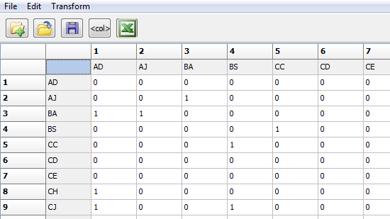
In the example, we see that node “BA” said that they were acquainted with node “AD.” But, note that “AD” does NOT indicate that they are acquainted with “BA” (read across the rows). Relational data are stored in square node-by-node matrices. Data may be “asymmetric” or “directed” (like the above example) where A→B does NOT necessarily imply B→A. In asymmetric data, the source of the relation is the row, and the destination of the relation is the column. Data may also by “symmetric” or “un-directed” or “bonded” where A→B does imply B→A. The diagonal cells (AD to AD, etc.) are usually ignored in SNA. It is conventional to code them as zero.
Social networks that have large numbers of actors can produce very large square matrices which can be difficult to edit, store, and process. Another very common way of recording relational data is the “edge list.” An edge-list is a list of the dyadic relations that are present in the social network (leaving out those that are absent). An edge-list contains the identity of the origin node and destination node for a directed tie (or the two nodes involved, in any order, in a symmetric tie), and the value of the tie. Many network analysis software packages are able to work with edge-list data (they convert it to full matrices for analysis). Statistical packages, when working with relational data, usually define each row of data as an “edge” (but they will also require a listing of the edges or relations that are absent).
The entries in a relational dataset may be binary, multinomial, ordered, or interval-ratio. Relations between the nodes in each dyad commonly represent the presence/absence of a tie, or what “type” of tie exists, or the strength or probability of a relation. Appropriate statistical treatment of relational data, of course, depends on the way that the relational variable has been measured. Most of our examples will be very simple, focusing on the simple presence or absence of a tie.
Individual nodes in SNA can have any number of attributes. These are stored in the dataset as one or more rectangular (node by attribute) matrices, or one or more vectors. Similarly, a SNA dataset can have any number of relational variables. Let’s consider some of the major types of relational variables used in many SNA applications.
2.3.1 Building Relational Variables from AttributesIn SNA, our focus is often on the existence, strength, or quality of the relationship between two nodes. Sometimes it is helpful to characterize the relationship between two actors as a function of the comparison between the attributes of each.
In SNA, the relationship between two nodes is “nested” within the pair of nodes. As an example, suppose that Fred is a man and Susan is a woman. We might wish to characterize the relation between Fred and Susan as being between two persons that differ on gender. That is, the dyadic relation between Fred and Susan is not gender homophilous.
The attributes of individual nodes are often important in SNA, but the more common SNA questions concern the comparison of the attributes of two nodes, which describes the dyad. One can imagine an analysis that uses attributes in both ways. For example, are women (individual level variable) more likely than men to have ties to persons of the same gender (a relational characteristic)?
UCINET has an interesting tool for comparing the attributes of two individual actors and building a dyadic variable (a relational variable that exhibits properties of dyads typically displayed in matrix form like the data in Figure 2.6) to describe the relation between them. Consider the dialog box created by Data>Attribute to matrix, shown as figure 2.7.
Figure 2.7. UCINET Dialog for Converting the Attributes of Pairs of Nodes to a Dyadic Variable
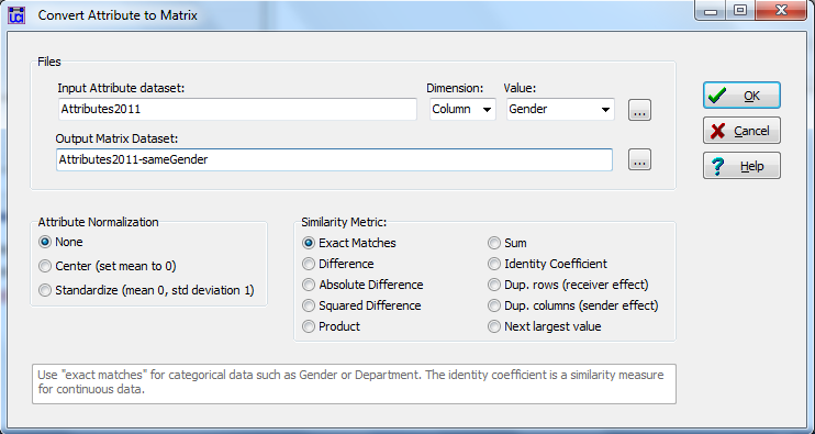
In this dialog, we’ve identified our rectangular attribute data set as input. We’ve selected the column (rather than the row, because our data array is actors-by-attributes, not attributes-by-actors), and the individual attribute “Gender.” The output of this procedure will be stored in a new dyadic (node-by-node square matrix) data set. In this case, we’ve selected “Exact Matches” in the “Similarity Metric” panel. This means: if the score of node A on the variable gender is the same as the score of node B on the variable gender, then code a “1” in the new matrix element AB (and BA). That is, the result of this operation is to build a matrix with “1” if two nodes are the same gender, and “0” if they are not. That is, a matrix of “gender homophily” is created.
There are a number of other useful functions here. “Difference” generates a “1” if two nodes are dissimilar. Absolute and squared differences measure the distance between two nodes on a quantitative attribute. Product and Sum generate a characterization of the dyad that aggregates their attributes. For example, we might think that the importance of the tie between two actors A and B is the synergy or multiplication of the degree of each of the two individuals.
The dialog also provides for normalizing the results (usually used with quantitative attributes). One may also automatically center the resulting dyadic score. This is often used in multi-level analysis to center the scores on the “level-1” (dyadic) variable around their mean.
2.3.2 Repeated MeasuresSNA work has increasingly focused on studying the processes that generate and modify network structures over time. While some research designs and data sources allow us to identify the exact time at which each dyadic relation is created or modified, most data sets consist of panel data – observations on the state of the dyadic ties as multiple, discrete, points in time. Our example data set, for instance, observes the ties among pairs of 75 students at four discrete times during an academic term.
Data on the same relation among the same actors is stored as a series of square node-by-node matrices in UCINET (with identical node labels and the nodes in the same order). For convenience in processing and displaying repeated dyadic measures, the matrices can be “stacked” into a single file.
Data>Join>Join Matrices combines or stacks multiple matrices with the same rows and columns into a single file. Subsequent runs in UCINET procedures will process all the matrices in the stacked file, and produce analyses for each matrix.
Another UCINET tool can be used when the multiple observations are missing some of the actors. This circumstance might arise where the data are taken from observations or documents at different time points, each of which reports on the actors present at the particular time of observation. Social network data are often collected by querying the actors who happen to be present at a particular time point, and each matrix may not include all of the actors who were ever present. If we want to include all actors in the analysis of each panel, we can use the time stack tool to build conformable data sets for each panel.
Transform>Time Stack has a dialog box that looks like Figure 2.8.
Figure 2.8. UCINET Dialog for Merging Dyadic Panel Data
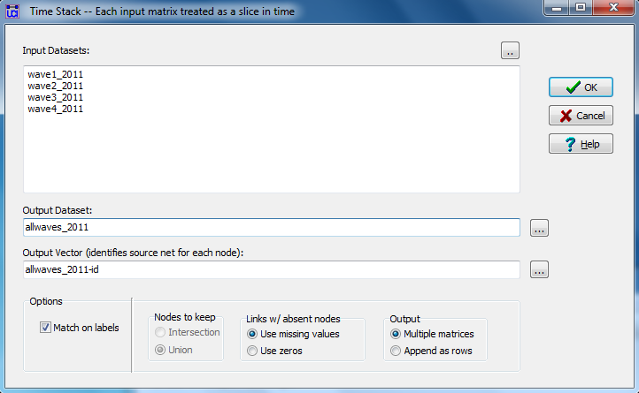
We’ve identified the student-by-student acquaintanceship at each of the four time points as our source data, and chose to save the data in a new file called “allwaves_2011” for future use. The default “Match on labels” has been selected for UCINET to determine which cases match across files. We’ve asked that missing value codes be entered for cases that are not present in a particular file (alternatively, one might want to assume that the case was present, but had no ties, by selecting “use zeros”). The output file or files will contain rows for all nodes that are in any of the input files.
When repeated measures have been joined into a stacked matrix in this way, another tool can be used to create a new dyadic variable that identifies change in ties. Tie change matrices can be interesting descriptively (e.g. did tie additions, i.e. new acquaintanceships, accelerate in the period of cramming for the final exam compared to other times in the quarter?). Tie changes can also be used as a dependent variable to test hypotheses about network change (e.g. are women more likely than men to form new ties?).
Transform>Build tie change matrices generates a dialog like that in Figure 2.9.
Figure 2.9. UCINET Dialog for Generating Tie Change Data
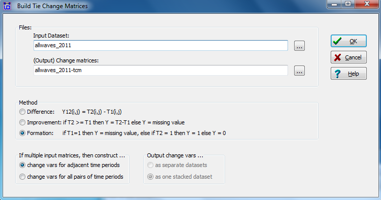
The input dataset is our time stacked data, and we can select a name for the matrices that result from the operation. The “Method” choices allow generating measures of any “difference” between two matrices (and it’s amount, if the relation is quantitative); or, we can select “improvement” to record only positive changes; or we can select “formation” to capture cases where there was no tie at time one, but a tie was formed by time two. One can also select whether the resulting stacked change matrices are calculated for adjacent points in time only, or for all pairs of time points.
2.3.3 "Training" NetworksThe relationship between two actors may be a function of a different relationship between them. In our example data, the students in the class were placed (more or less randomly) into groups to work on research term papers. An obvious hypothesis would be that being placed into the same research team will result in becoming acquainted with other team members (actually, this didn’t always happen in the class!).
This is an example of one network (who shares the relation of “being in the same work group with”) that “trains,” or acts as a “context” or “social geography,” that may guide the formation of new acquaintanceship ties. Being present in the same physical space, being members of the same organization, and other forms of affiliation can modify the likelihood of ties of other types forming.
Similarly, if one type of tie exists between two nodes (say, one goes to the other for advice on the job), this may modify the likelihood of the formation of another kind of tie (say, being friends outside of work). In a slightly different sense, the presence of one kind of network tie (advice seeking) is “training” the other network (being friends).
Network data that describe the presence of joint affiliation, or context, or other kinds of ties are recorded just like any other network or relational variable – as a square matrix (node-by-node, directed or not, valued or not). As we will see later, the relation between two nodes in one (training) network can easily be used to predict the relation between the two nodes in another.
One of the most important strengths of the way that SNA conceptualizes social structure is in recognizing how contexts shape (and are sometimes shaped by) patterns of ties between pairs of social actors. The most often cited example of this idea is the study by Davis, Gardner, and Gardner (1941) of sociability among a group of women in a southern town. Davis et al. recorded whether each of the women had attended each of a number of social events. The strength of ties between pairs of women can be indexed by the number of events they both attended (and/or both did not attend).
Data structures that show the ties between two types of social entities (in the Davis et al. example, women and social events) are called “two-mode” (or “bi-partite” or “affiliation”). The data are usually recorded as a rectangular matrix of actors (on the row) by events (on the column). For use in our statistical analyses where we are predicting dyadic outcomes, affiliations need to be turned into node-by-node matrices. The idea is simple: the tie between two nodes is some function of the pattern of their affiliations. Usually, if two actors have very similar affiliations, we regard the tie between them as strong; if they have very dissimilar affiliations, we regard their tie as weak.
In many social network analyses, it can be very important to create dyadic variables that measure shared context or joint affiliation between the members of dyads. Such variables often represent the similarity of the locations of the actors in “social space” and can be strong predictors of the likelihood of other kinds of social ties between them.
There are a variety of approaches and tools for turning affiliation data into dyadic variables for use in SNA. Here are just a few:
Sometimes we have stored information about context or affiliation as a vector. In our student data, for example, we recorded which of 10 workgroups a student was assigned to. We might want to turn this into a student-by-student dyadic variable, coded as “1” if two students were in the same workgroup and “0” otherwise. The UCINET tool Data>Partition to sets will help to accomplish this task, as in figure 2.10.
Figure 2.10. UCINET Dialog for Partition to Sets

In this dialog, we’ve opened our “attributes” file (nodes by attributes), and told UCINET to use column 3, which (from our codebook) we know to be the “work group number” variable. We’ve given a new name to the output file. The output dialog is shown in Figure 2.11.
Figure 2.11. UCINET Output of Partition to Sets
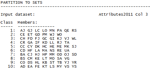
The output data file that we called “Same_work_group”, a portion of which is shown in Figure 2.12, is a node by attribute “affiliation” matrix. That is, it shows, for each student, whether they were a member of group 1, group 2, …, group 10, with dummy codes.
Figure 2.12. UCINET Output Data from Partition to Sets
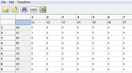
These 10 dummy variables could be treated as “level2” (individual) attributes in a multi-level analysis.
We may also want to create a dyadic variable to represent co-presence in the same work group; this is a dyadic or “level 1” variable. To convert the “Same_work_group” data file to a student-by-student dyadic variable, we can use the Data>Affiliations (2-mode to 1-mode) tool. The dialog is shown in figure 2.13.
Figure 2.13. UCINET Dialog for Affiliations: Convert 2-mode to 1-mode Data
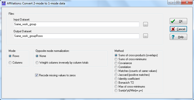
We’ve input our affiliation matrix of students by workgroup dummy variables, and accepted the default output name (“Same_work_groupRows”). This UCINET tool has many useful options. We can choose to work on either rows (to create student-by-student output) or columns (to create a workgroup-by-workgroup matrix). We can normalize output (useful when the input is quantitative rather than binary), and insert zeros for missing data. There are also many useful choices about how to define “affiliation.” The “sums of cross-products” multiplies each element of the work-group membership of one person by that of the other person, and sums the result. With binary data, and only one group membership for each actor, this creates a matrix where a pair is coded “1” if they are in the same work group, and zero otherwise. The other options provide alternative ways of operationalizing the idea that two actors have more “similar” affiliations or stronger ties.
The output file that results from this dialog is shown as figure 2.14.
Figure 2.14. UCINET Output of Affiliations Tool
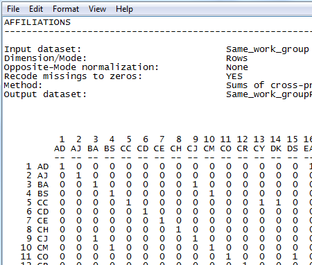
The output file is a binary, symmetric matrix. We see that BA and CJ are coded as being in the same group, for example. This dyadic variable can now be used to test group difference between workgroups.
The “affiliations” tool is particularly useful when we want to define the similarity, or closeness, or strength of ties between members of a dyad based on the profile of ties that they have with contexts, attributes, identities, or other social objects with which social actors can affiliate.
More generally, we may wish to create dyadic variables describing the strength, closeness, or similarity between members of dyads based on the similarity of their profiles across any set of attributes. For example, one might have information about the location of each actor in “Blau-space” (e.g. their gender, ethnicity, social class, education, etc.; McPherson & Ranger-Moore, 1991). We might wish to reduce this complexity to a single similarity score to characterize the social closeness (the inverse of social distance) between the actors in each dyad. Such similarity is often important in promoting the formation of social ties.
Any number of techniques can be used for this kind of scaling of actors. We begin by comparing each pair of actors, and calculating a similarity or a distance between them based on their scores on multiple attributes. UCINET provides two suites of tools for generating similarity or distance matrices: Tools>Similarities and Tools>Dissimilarities & Distances.
Once an actor-by-actor similarity (or dissimilarity) matrix is created from the attribute vectors, it can be used directly as a dyadic variable. Similarities and distances between actors can also be further reduced and refined by using clustering and/or scaling (Tools>Clustering; Tools>Scaling/Decomposition).
When other relational variables serve as independent variables in an analysis of a relational dependent variable, they present no special challenges. For example, we might be interested in the extent to which the relational variable “respondents are the same gender” predicts the outcome “respondents have a reciprocal acquaintanceship relation.” But there are occasions when we may be interested in more than one relational variable as dependent. For example, we might seek to explain both “friendship” and “advice seeking” as functions of independent variables.
In conventional statistical analysis, multiple dependent variable problems lead us into the territories of simultaneous equations or structural equation modeling. Unfortunately, specifically tailored applications of these techniques don’t exist for relational outcomes (as of this writing).
When the problem calls for the treatment of multiple relational variables as dependent, there are a number of choices, all of which have some difficulties.
One can analyze each outcome separately, using the other outcomes as independent, along with other predictors. Of course, this is a mis-specification, and also does not deal with possible correlated errors across the multiple dependent relational variables.
Alternatively, one can scale the multiple outcomes with mathematical or logical operations. For example, if two actors are both friends and advice givers, we might code the dyad “2”; if either relation is present, we might code “1”; if neither relation is present, we would code “0.” Or, we could treat the outcome as the presence or absence of each of 4 types of relations (both ties present, only friendship present, only advice giving present, neither present). Ordered outcomes (such as the 0, 1, 2, 3 coding) or multinomial coding (such as treating each combination of relations as a qualitative type of tie) can be analyzed in some multi-level statistical software that will do hierarchical modeling with non-Gaussian dependent variables.
Several groups of researchers have made continuing contributions to the development of statistical analysis of network data. As of this writing, there are a number of very interesting and useful packages that have been made freely available to network modelers (Huisman and van Duijn, 2011). UCINET and several other packages (e.g. Pajek) have excellent suites of tools for describing and working with univariate and bi-variate network and attribute data. Multivariate analysis in the generalized linear modeling framework has been developed in specialized (and free) packages such as Stochnet, Statnet, PNET, ORA, and Sienna (http://www.gmw.rug.nl/~stocnet/StOCNET.htm; https://statnet.csde.washington.edu/; http://www.melnet.org.au/pnet/; http://www.casos.cs.cmu.edu/projects/ora/; https://www.stats.ox.ac.uk/~snijders/siena/). Most recently, software development for Exponential Random Graph and related statistical modeling has been prepared for the R environment (https://cran.r-project.org/web/packages/statnet/index.html; https://cran.r-project.org/web/packages/sna/index.html; https://cran.r-project.org/web/packages/ergm/index.html; https://cran.r-project.org/web/packages/RSiena/index.html).
The data structures that we’ve discussed above are common to all of the specialized packages for the descriptive and predictive analysis of network data – though the details of how data are prepared vary somewhat from package to package.
Many (but not all) multivariate predictive analyses of network data can also be carried out with standard commercial statistical software such as Stata and SAS. Because these packages were primarily designed for non-network analysis, they require a rather different data structure. We’ll discuss, and show an example of preparing and analyzing relational data with Stata in Chapter 8.
Social network analysis often involves the description and explanation of attributes of nodes. Working with nodal attribute data is similar to conventional statistical approaches that analyze attributes of cases at the individual level. Often, social network analysis will treat network position or structural measures of embeddedness as individual level data using them as predictors or determinants of nodal attributes.
Unlike conventional analysis, social network analysis also involves the description and explanation of relational data. Unlike traditional rectangular data arrays, relational data is often represented in square matrices and contains information about dyads or pairs of nodes. Relational variables often display the presence/absence or strength of ties between pairs of nodes. Additionally, relational variables can be generated using nodal attribute data (e.g. the degree to which both nodes in a dyad share a given attribute) and are often used to represent shared affiliation.
This chapter introduced an example dataset that was used to display different types of network data. The dataset contains acquaintanceship information about 75 undergraduate students from four points in time across a single course term and will be used throughout the rest of this text to demonstrate a variety of social network analytic techniques that deal with nodal attribute data, relational data, and both simultaneously.
Davis, Allison, Burleigh Gardner, and Mary Gardner. 1941. Deep South: A Social Anthropological Study of Caste and Class. Chicago: University of Chicago Press.
Huishman, Mark and Marijtje A J Van Duijn. 2011. “A Reader’s Guide to SNA Software,” Pp. 578-600 in The SAGE Handbook of Social Network Analysis, edited by J. Scott and P. J. Carrington. London: Sage.
McPherson, J. Miller and James R. Ranger-Moore. 1991. “Evolution on a Dancing Landscape: Organizations and Networks in Dynamic Blau Space.” Social Forces, 70(1): 19-42.