Chapter 6. Network Influences on Attributes
A key insight of SNA is the seemingly obvious idea that an individual’s attitudes and behaviors are affected by the attitudes and behaviors of those to whom the actor is connected. In order to understand or predict ego’s attributes then, we need to take processes of social learning and social influence into account. The processes of learning, influence, and diffusion are all action on social networks.
In this chapter we’ll look at some ways that social influence can be incorporated into statistical models that predict individuals’ attributes and behaviors as outcomes. Models of this type include both the individual’s own attributes, and the attributes of those to whom an individual is tied to as predictors. Models of how an individual’s attributes may affect outcomes are commonplace, if not important. For example, women may be more likely to vote than men. What social network analysis adds to explanations of this type are the effects of social learning and influence. For example, while women may generally be more likely to vote than men, women who have more friends that are women might be even more likely to vote than those who have less gender homophilous networks.
The challenges of including information about ego’s network in explanations of ego’s behavior are more conceptual and theoretical than they are methodological. Models of individual outcomes for actors embedded in networks use individuals as units of analysis, and use conventional general linear modeling approaches. Data about how ego’s network affects ego’s behavior are included as attributes of ego – though they measure structural properties of the graph. For example, assuming that gender is predictive of voting behavior, when explaining whether a person votes or not, one might very well want to include information about the size of ego’s friendship network as well as the proportion of women in their friendship network.
In many cases, the most important attribute of ego’s network is whether the alters in the network display the behavior or attitude in question. If we want to explain variation in voting, we would probably hypothesize that as the number or proportion of ego’s neighbors who vote increases, the likelihood that ego will vote increases. The technical term for this is “network autoregression.” This is the tendency for a node to have scores on the dependent variable that are more similar to those of their network neighbors than to random others as a result of causal processes (social learning, influence, diffusion, etc.). Network autoregressive processes are modeled by including measures of the prevalence of the outcome in ego’s neighborhood. Sometimes we may wish to include indirect, as well as direct influences. For more complex processes operating over broader social space, “spatial lag” models may be helpful.
There is also the possibility that a positive autocorrelation between ego and ego’s close neighbors arises from local “error” or unobserved latent variables affecting both ego and alters. One may overstate the significance of autoregression (social learning or influence) in the presence of spatially autocorrelated error.
Below, we’ll first take a look at some common approaches to incorporating information about how an individual is embedded in a network into models predicting an individual’s attitudes or behavior. Many social learning and social influence processes that operate only locally to produce autoregression can be specified fairly easily. For influence processes that operate over somewhat broader social spaces, we may wish to borrow spatial autoregressive modeling approaches from econometrics and geostatistics. And, finally, we’ll take a look at how spatially autocorrelated error or mis-specification can be controlled.
Setting up the data for analyses that predict the attributes of nodes is fairly straightforward. Most analyses represent independent variables as attributes of the individual, and use regular generalized linear modeling, with permutation test approaches to assess significance. We’ll talk first about some typical kinds of predictor variables such as other attributes of the individual along with measures of how they are embedded in the network. Then we’ll discuss spatial weights, which are necessary for social-spatial autoregressive and autocorrelated error models.
6.2.1 Dependent Variables: Levels of Measurement and Distributional ShapesModels of network influence usually focus on some time-varying attribute of individuals, such as attitudes, behaviors, or conditions. We might be interested in examining the role of network influence on attitudes toward some issue. Do people who have many friends who believe that the earth is flat, also tend to believe it is flat? Sometimes behaviors are the focus. Are students who are friendly with other students who have poor academic performance more likely to perform badly themselves? And, sometimes we might focus on some kind of material condition. Are the social networks of people who own Lamborghini automobiles likely to contain others who also own these? Recently, and controversially, it has been suggested that happiness and depression may be transmitted by way of social networks.
The outcome in our models is an attribute of individuals, and can be scaled at any level of measurement. Depending on how the dependent variable is measured, appropriate versions of distributional family and link functions of generalized linear models can be used (except for spatial autocorrelated error and spatial autoregression models which have somewhat more limited software at this writing). In our examples, we’ll focus on two measures of the academic success of our students. As a binary measure, we’ll examine which factors may affect whether the student passed or failed the final exam (that is, earned a grade of 70% or more). As a continuous measure, we’ll focus on the same final exam, but analyze the actual score earned.
6.2.2 Independent Variables: AttributesConventional (non-SNA) models of attitudes and behavior focus on individual level factors as predictors. For example, men and women may be expected to differ on an outcome, people of different ethnicities or religions may be hypothesized to vary, etc. Individual attributes are used in social influence analyses in exactly the same ways, and there is nothing much more to say about them here. Individual attributes are simply coded and entered as they might be in any other analysis (see Chapter 3).
In our student data that we introduced in Chapter 2, we don’t have very much information about the individual attributes of the students. Only self-identified gender and ethnicity were recorded. We might predict that women students would out-perform men students on the final exam in our class, as they tend to do in most classes, due to differential socialization and selection processes that occurred prior to entering our course. Similarly, we might expect differences by ethnicity.
6.2.3 Independent Variables: Measures of Network EmbeddingConventional analyses of an individual’s attitudes and behaviors rarely pay much attention to explicitly measuring variations in an individual’s social networks. SNA, of course, focuses on describing and indexing variation in the ways that individuals are embedded in networks. People who have many friends may be easier to reach with a message than those who are less connected. Actors who are tied to others who are tied to one another may be more difficult to convert because of strong countervailing pressures. Actors who are embedded in networks that are highly homophilous may be more subject to conformity pressures. Actors who are key-players, or central and prominent figures in networks, may be more likely to have conventional attitudes and behaviors.
Social influence models may include a number of different measures about how an actor is connected as predictors of their attitudes and behaviors. Just like the attribute variables discussed above, these measures of network embedding are nodal variables describing the ways in which the nodes of a network are embedded. The authors of the UCINET software have provided tools that are useful for building variables that describe how nodes are embedded in the network. Taking a brief look at these tools suggests some common types of network-contextual variables that one might want to include in an analysis. The UCINET tools also have the advantage of calculating numerous network measures that are saved as files, and can be appended to our attribute file for use as predictors.
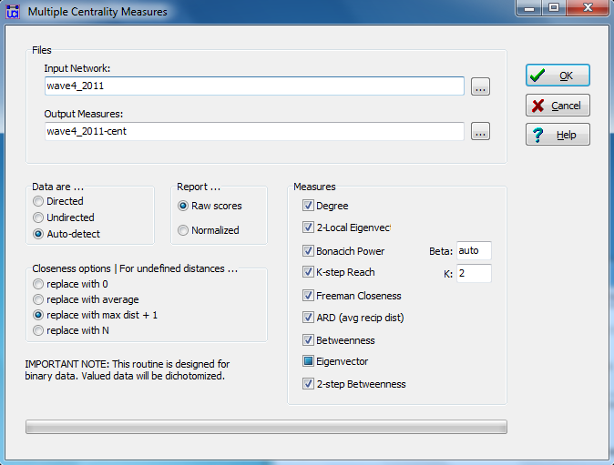
Network>Multiple Measures> Node Level produces a number of measures of how connected nodes are, their distance from other nodes in the network, and their centrality (defined in a variety of ways). Figure 6.1 shows the dialog.
Figure 6.1. UCINET Dialog for Node Level Measures of Network Embedding

In the dialog, we’re using the student data introduced in Chapter 2. We’ve specified that the input file is the acquaintanceship network at the time of the course final exam (wave 4). Since we will want to save the output and append it to the file of individual attributes, we’ve used the default file name for the output. We could specify the data as directed, or let the program detect that it is (auto-detect) given the fact that the acquaintanceship matrix is asymmetric across its diagonal. UCINET can calculate normalized scores, which may be useful for comparison across different networks. Since we are only concerned with the one class, we’ll keep the original metrics (note “Raw scores” is selected). The last panel (lower right), lets us choose various measures of distance and centrality, which we will discuss with the output that is shown in Figure 6.2.
Figure 6.2. UCINET Dialog for Node Level Measures of Network Embedding

The number of ties actors have to others in the network, and how close they are to others, could affect whether they adopt an attitude or behavior. From the output in Figure 6.2, we see that AJ has fewer connections than actor BA, both from others naming them as acquaintances (in degree; column 1) and others that they’ve named (out degree; column 2). UCINET also provides measures of out degree and in degree of an actor’s direct acquaintances. In column 3, Out2local tells us the total number of acquaintances named by each acquaintance named by ego. For example, because the out degree of AD is equal to four, we know AD named four others as acquaintances (whether they named AD or not). The total number of others named by those four is captured by Out2local and is equal to 48. Similarly, In2local (column 4) tells us the number of acquaintances that named the acquaintances of ego. So because 17 students named AD as an acquaintance (in degree = 17), we know those 17 were named as acquaintances 259 times from In2local.
The local two-degree measures just discussed seem a little odd. We know there are only 75 students total in the data set, yet the 17 in degree acquaintances of AD were named 259 times? This is due to the potential for repetition in naming others (e.g. multiple students might name all 17 students that name AD, generating a large value of In2local). If instead we are interested in the unique number of students that are separated from ego by two steps (“friends of my friends”), we can look at Out2step (column 7 in Fig. 6.2) and In2step (column 8). For example, though the 17 students that name AD are named 259 times, there are only 69 unique students that name them (In2step). So AD is connected to 69 of the 75 students in the class by only two steps of separation, at least for inward ties (pointing toward AD). AD is only connected to 35 students via two steps of outward ties (Out2step).
The average distance from ego to all others in the network that are reachable (OutARD, column 9 in Fig. 6.2) and the average distance to ego from all others in the network that can reach ego (InARD, column 10) are provided. Also, included are Outclose (column 11) and InClose (column 12). OutClose tells us the out-closeness which can be thought of as the degree to which ego can reach all other nodes in the network via short path lengths. In-closeness, then, is the degree to which ego can be reached by all other nodes via short path lengths. All of these measures are possible ways of thinking about the density or closeness of each actor to the broader network. Social influence models often hypothesize that actors who are more connected, in one way or another, are more likely to have attitudes and behaviors that are closer to the mean or mode.
The output also shows measures of ego’s centrality in the network. The Bonacich power measures (as well as a similar measure that’s not shown, the eigenvector centrality) indicate whether ego is connected to other well-connected actors. If ego has high in-centrality (e.g. column 6 in Fig. 6.2), i.e. they are being influenced by other influential actors, they may be “constrained.” If ego has high out-centrality (column 5), they are able to exert influence on other influential actors. Actors who have high “betweenness” centrality (columns 13 and 14) are acting as transmitters or brokers of ties between other pairs of actors. Being a “broker” may be a source of power, and hence make an actor less constrained and more influential.
For many social processes, the way that an actor is embedded in their local neighborhood of the social network can be more important than their overall centrality or distance from others. UCINET has a number of tools for describing ego-networks (the actors that are connected to ego at a short distance, and the connections among them). Metrics on each actor’s ego-network can provide some interesting insights into variation in ego’s attitudes and behaviors.
Network>Ego Networks>Egonet Basic Measures in UCINET allows varying definitions of neighborhoods, and calculates a number of measures describing the topology of each node’s local network. Figure 6.3 shows a dialog for the acquaintanceship data at the time of the final exam.
Figure 6.3. UCINET Dialog of Basic Egonet Metrics for Wave 4 Acquaintanceship

In the dialog we’ve identified the acquaintanceship matrix at wave 4 (the time of the final exam). Since the network is directed, we can choose to define it by relationships directed at ego (the in-neighborhood), relationships from ego to alters (out-neighborhood), or to include both. We’ve chosen to define ego’s neighborhood as any actors that claim ego as an acquaintance (and any ties among these alters). The in-neighborhood is a reasonable choice because we are focusing on how ego is influenced by alters (rather than how influential ego is with alters). The output dataset was named and saved to be used later, so that it can be appended to the attributes dataset to act as a set of independent variables for predicting ego’s attributes. Figure 6.4 shows the output for the first 10 of 75 egos.
Figure 6.4. UCINET Output of Basic Egonet Metrics for Wave 4 Acquaintanceship

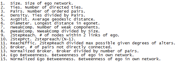
Most of the common metrics for ego-networks (egonets, for short) get at the same ideas as the global measures we saw above. Student AJ, for example, has 7 students who name him/her as an acquaintance (column 1 in Fig. 6.4). Among those 7 others (not including AJ), there are 42 possible ties (column 3), of which 26 are actually present (column 2). The density of ego’s local neighborhood, then, is 61.9% (column 4).
The density of an egonet, leaving ego out of it, is also called the “clustering coefficient,” and it is often useful as a measure of the “open-ness” of ego’s network. If ego is known by others who are connected to one another, we may observe “clique” like pressures for conformity and resistance to outside influences. If ego’s network has low clustering, or is an “open” network, ego may be exposed to more diverse and competing pressures. The “granularity” of ego’s local network, or the extent to which it is composed of groups of connected others, is also commonly indexed by the ratio of the number of weak components (groups of alters, all of whom are connected to one another; column 7 in Fig. 6.4). How close ego’s network is to the network as a whole can be seen by looking at the percentage of all nodes that are within two steps of ego (the first step is in ego’s local network, the second step reaches beyond; column 9). The “reach efficiency” measure (column 11) also addresses the idea of the open-ness of ego’s network. The efficiency measure tells us the amount of contact ego gets with the larger network per member of ego’s personal network. Low ratios indicate more network closure.
The last four measures deal with ego’s influence or power in their local neighborhood. It is assumed for egonets that ego has more influence and greater autonomy to the extent that he/she controls the access of other members of the network to one another. Brokerage (column 12 in Fig. 6.4) and betweenness (column 14) are alternative ways of indexing the extent to which alters in ego’s neighborhood are dependent on ego. Some additional measures of ego’s autonomy and influence derived from Ronald Burt’s work (1992) are available under Network>Ego Networks> Structural Holes. Some measures of the role that ego plays in connecting groups of actors with different attributes (e.g. acting as a “gate keeper” in relations between White and Asian students), developed by Gould and Fernandez (1989), are available under Network> Ego Network> G+F Brokerage roles.
The measures of ego’s local network that we’ve looked at so far refer to its structure and ego’s embedding in it. It may also be very important to understand the composition of ego’s network (e.g. is ego tied to mostly women, or mostly to men? And, to what extent is ego tied to alters who are similar or dissimilar to ego, i.e. homophily?). UCINET has some helpful tools for constructing measures of network composition and homophily of the local context of each actor. These indexes can also be saved and appended to the attributes dataset.
Figure 6.5 shows the dialog for Network>Ego Network>Egonet Composition>Categorical Alter Attributes which can be used to build measures of the attributes of the others in ego’s one-step neighborhood. There are two versions of this tool. One works with categorical alter attributes (like the gender or racial compositions of those tied to ego); the other with continuous alter attributes (like the average attendance rates or test scores of those tied to ego).
Figure 6.5. UCINET Dialog for Generating Egonet Composition Measures (Categorical Alter Attributes)
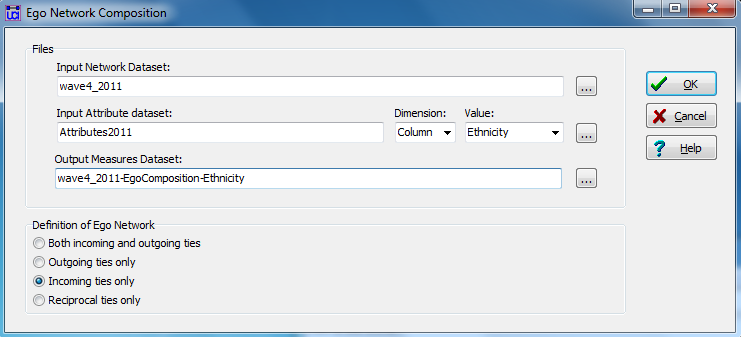
In this dialog, we focus on the acquaintanceship network at the time of the final examination and identify the attributes dataset and column that contains ego’s ethnic identity. If we are interested in the social composition of actors who are influencing (rather than being influenced by) each student, we can select “incoming ties only.” Figure 6.6 shows a portion of the results which are saved as a file that can be appended to the attribute file. We will save the output measures to be used later.
Figure 6.6. UCINET Output of Egonet Composition Measures (Categorical Alter Attributes)
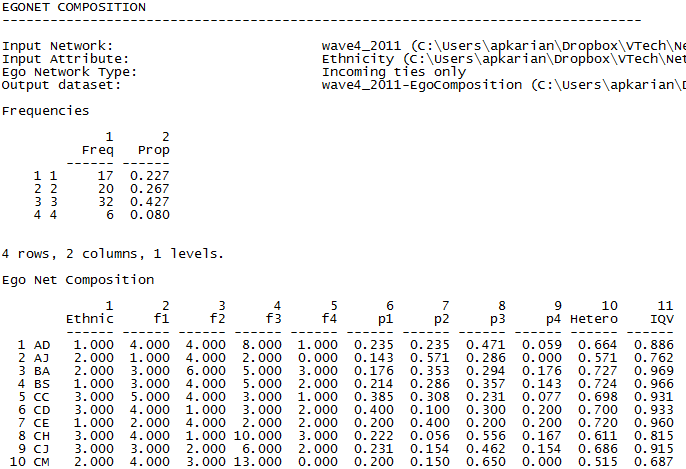
In the above output, ethnicity = 1 refers to White, ethnicity = 2 refers to Hispanic, ethnicity = 3 refers to Asian, and ethnicity = 4 refers to African American. We see from the frequency table that the network as a whole is composed of 17 Whites, 20 Hispanics, 32 Asians, and 6 African Americans. From the first column, we can see that actor AJ identifies as Hispanic. AJ is identified as an acquaintance by one White student, four Hispanic students, two Asian students, and zero African American students (columns 2 through 5). The next four columns display the proportion of total incoming ties from students of each ethnic identity. One summary measure of heterogeneity (column 10 in the output) was developed by Peter Blau, and is described in UCINET as “1 minus the sum of the squares of the proportions of each value of the categorical variable in ego's network. For example, a person connected to equal numbers of men and women will have a Heterogeneity measure of 0.5, calculated as 1 - ( (1/2)^2 + (1/2)^2) ).” This value can be thought of as a non-normalized index of qualitative variation (the interpretation varies by the number of categories of the discrete variable being measured). The last column provides the index of qualitative variation (column 11). Both measures suggest moderate heterogeneity in the ethnic identity of students who influence AJ.
Figure 6.7 shows the dialog for indexing the composition of ego’s neighborhood on a continuous attribute. In this case, the rate of participation in the term paper project as assessed by members of the student’s work group.
Figure 6.7. UCINET Dialog for Generating Egonet Composition Measures (Continuous Alter Attributes)
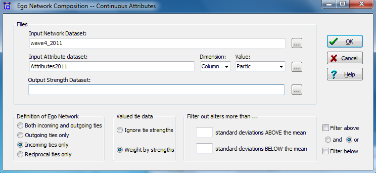
As usual, we identify the network from which we want to extract the egonets (acquaintanceship at wave 4), and the file and column containing the student’s attribute of participation grade in the final project. The output might be saved for appending to the attribute file. We’ve selected “Incoming ties only” to focus on the attributes of alters who are influencing ego. If the network was a valued network (e.g. “on a scale of 1 to 10, how well do you know X?”), we could weight the attributes of the alters proportional to tie strength (our network, however, is just a binary zero-one). Since the output will be means and standard deviations, alters with extreme scores could skew the results. Options are available to trim means and standard deviations. The output is shown in figure 6.8.
Figure 6.8. UCINET Output of Egonet Composition Measures (Continuous Alter Attributes)
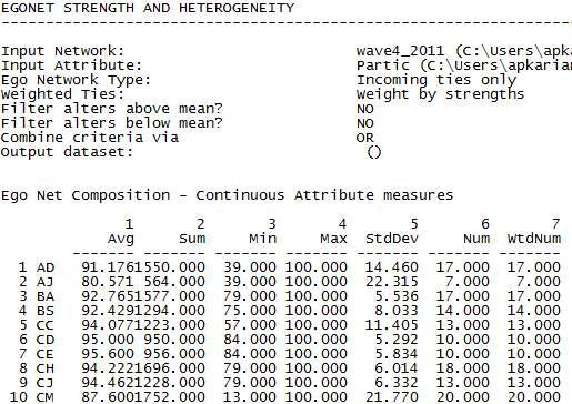
The first two columns appear to bleed into one another. Keep in mind that this command rounds to three decimal places, so the first column for AD reads 91.176 and the second column reads 1550.000. We can see from the output that AJ was identified as an acquaintance by seven others (column 6), all of whom were rated as not very active participants in the term project (average of 80.6 out of 100 possible; column 1). Their scores were also very diverse ranging from 39 to 100 with a standard deviation of 22.3. Actor CD, on the other hand, was being influenced by 10 alters who had a much higher average participation rate (95.0), who were also much less diverse in this regard (ranging from 84 to 100, with a standard deviation of only 5.3).
The ego-net composition tools are potentially quite important in the analysis of social influence, as they enable us to index the attributes of those who are directly connected to ego in the network. We may be interested in both the central tendency (what kind of alter is typical for ego? what is the mean or average score of the alters of ego?), and in diversity or variation among the alters.
Building on this idea of homogeneity or diversity of the attributes of those influencing alter, SNA particularly focuses attention on “homophily” or the extent to which ego is similar to alters. Students who are tied to other students who are very similar to themselves may be more subject to stronger constraints but may also have higher levels of social support. UCINET, again, provides a fairly convenient tool for indexing the homophily of ego’s network with Network>Ego Networks>Egonet Homophily. A dialog for this tool is shown in figure 6.9.
Figure 6.9. UCINET Dialog for Generating Egonet Homophily Measures
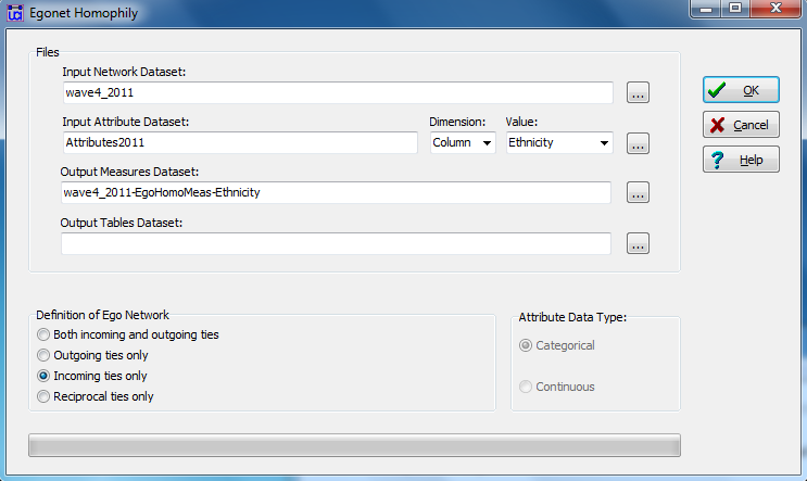
In this dialog, we’ve asked for measures of the similarity of the ethnic composition of ego’s network to ego’s own ethnic identity, using the acquaintanceship network at wave 4 to identify incoming tie egonets. As always, the results shown in figure 6.10 can be saved to a file, and then appended to ego’s attributes to be used later.
Figure 6.10. UCINET Output of Egonet Homophily Measures
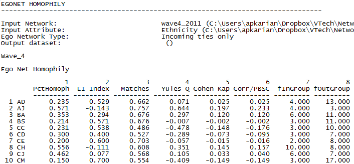
Various measures of the similarity of ego’s ethnic identity to that of his/her in-neighbors are given. The percentage of neighbors who have the same ethnic identity as ego (e.g. 57.1% for AJ) is the most obvious (column 1 in Fig. 6.10). The numbers of neighbors who have the same ethnic identity as ego (column 7) and different ethnic identity as ego (column 8) are displayed as well. The EI index (column 2) is the difference between the numbers of ties to actors outside ego’s group less the number of ties to actors inside ego’s group, divided by the total number of ties. Positive values, therefore, show a preponderance of “external” ties and negative values show a preponderance of “internal” or homophilous ties. A variety of other measures are provided that may be of interest, depending on the problem.
Unfortunately, as of this writing, UCINET does not have a tool for computing measures of egonet homophily for continuous attributes. For example, there is no simple tool for calculating an index of how similar ego’s score on group participation is to the participation scores of those who identify ego as an acquaintance. If this sort of homophily is important, one can recover the average score of ego’s alters on a continuous attribute using Network>Ego Networks> Egonet Composition>Continuous Alter Attributes, and calculate the difference of ego’s score from the mean of ego’s neighbors.
In this rather lengthy section we’ve looked at some ways of indexing how each actor is embedded in both the global, and their local (ego) network. How connected ego is, how central they are, whether or not their neighborhood is highly clustered and/or well connected to the global network may all be important structural aspects of an actor’s location that affect their attitudes and behavior.
Of course, it is not just being connected that matters. It may matter to whom one is connected. Indexing the attributes of the others in an actor’s neighborhood (composition), and measuring how similar an actor is to his/her neighbors (homophily) may also matter in predicting an actor’s attitudes and behavior.
6.2.4 Independent Variables: Weights for Network Autoregression and AutocorrelationThe attributes of those to whom an actor is connected may affect the actor’s attitudes and behaviors. Probably the most critical attributes of ego’s neighbors are the attitudes or behaviors that we want to understand. A key variable in network models of social influence then, is the values of the dependent variable for those who are connected to an actor. If we are trying to understand a student’s performance on the final exam, an important predictor may be the performance of those who are most influential via the student’s social network.
An actor’s score on the dependent variable may be influenced by the scores of their network neighbors via two different processes: autoregression and autocorrelated error. When the scores on the dependent variable of ego’s neighbors directly cause ego’s score we have “autoregression.” As in social influence or diffusion models, the scores of alters are treated as independent variables. Sometimes ego’s score on the dependent variable may be correlated with that of ego’s neighbors because of local disturbances or omitted variables. These kinds of error processes are called “autocorrelation.” Autocorrelation is treated as spatially correlated error, similar to time-correlated error in time series analysis.
Whether the process involved is autoregression or autocorrelation (or both), we need to represent the scores of alters on the dependent variable as a predictor or ego’s scores in network influence models. There are a variety of approaches.
First, one can simply summarize the scores of alters on the dependent variable directly. If we are only concerned with alters who are adjacent to ego, we can use Network>Ego Networks>Egonet Composition>Continuous Alter Attributes or Network>Ego Networks>Egonet Composition>Categorical Alter Attributes to create a new variable that is the mean score of alters directly tied to ego on the dependent variable, or the proportion of ego’s direct-tie alters that have a particular score on the dependent attribute. Figures 6.11 and 6.12 calculate the average score of direct-tie alters on the final exam for each ego, which we will use as an independent variable to predict ego’s score.
Figure 6.11. UCINET Dialog Used to Create Alters’ Average Score on the Final Exam
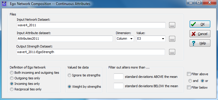
Figure 6.12. UCINET Output for Alters’ Average Score on the Final Exam
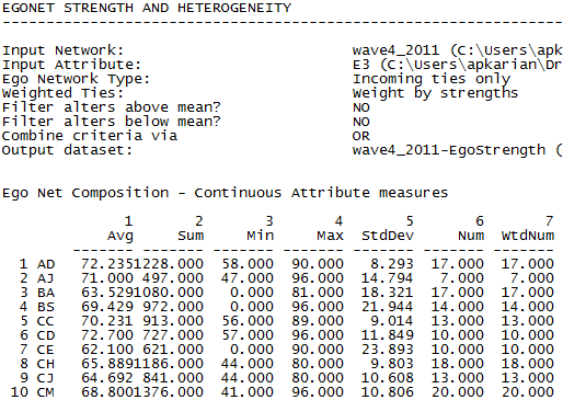
We see, for example, that AJ’s seven (column 6) in-neighbors had an average score of 71.0 (column 1) on the final exam, and that CJ’s 13 in-neighbors did worse with an average of score of 64.7. It might be worth noting (and possibly including as a predictor variable) the variation among the neighbors. While the neighbors of BS and CC performed similarly on the exam, on the average, the performance of BS’s neighbors was much more variable (see column 5).
For many autoregressive and/or autocorrelation processes, we may believe that neighbors who are more than one step from ego might have indirect effects on ego. Usually we believe that the influence of alters declines with distance from ego, and most often we think that this influence declines rapidly with distance.
For more complex ideas about the effects of neighbors at-a-distance, it is best to create a matrix of distance weights as we did in chapter 5 for calculating the Moran and Geary network autocorrelation. With a little matrix algebra and a distance-weights matrix, one can create an independent variable to use directly in modeling. Or, one can use the weights matrix in software designed for autocorrelated error and autoregression, as we do in an example later on in this chapter.
One common metric for social network “nearness” (or distance weighting) is the reciprocal of the geodesic distance between nodes. See Figure 5.11 (last chapter) to see these dyadic data nearness weights.
We now have all the pieces in place. Our dependent variable is a measure of some attribute of ego. Our independent variables include other attributes of ego, specifically, measures of the ways in which ego is embedded in the network globally and locally. We also use measures of the composition of ego’s neighborhood and ego’s homophily with the alters in ego’s direct-tie neighborhood as independent variables. Finally, we include measures of direct-tie alter’s scores on the dependent variable to measure any effects of autoregression and/or autocorrelation.
This sounds complicated. However, once the data are assembled, the analysis is an exercise in linear modeling, with the use of permutation to test hypotheses. Let’s look at a variety of approaches.
As we saw above, we can create measures for each actor that describe variation in their position in the network and the influences operating on them through their network connections. For example, an actor’s betweenness centrality might be used to get at the idea that actors who are more central in the global network are more likely to have more favorable outcomes because they have more dependent alters that they can draw on for resources. Or, actors who are embedded in local neighborhoods that contain many individuals who are similar to themselves and/or have high closure may perform more poorly because of the lack of diversity in the social capital that they have available.
Having created variables for each actor that measure not only their attributes, but also their structural location in the network and the influences operating on them, we can apply regular generalized linear modeling techniques to explain variation in individual attributes. This approach to understanding network influence on individual attributes has the advantage of being able to deal with actor outcomes that have a variety of distributional forms and a variety of link functions to the predictors.
Analyzing network influence this way treats each actor in the network as a case, but the cases are obviously not independent of one another. Consequently, permutation or other re-sampling methods should be used to assess the reliability of parameters. Let’s look at some examples.
Suppose that we are trying to predict a student’s performance on the final examination. We might treat the outcome (the individual’s performance on the final exam) in a variety of ways. Since a score of 70 or more was considered to be “passing,” we might dichotomize the outcome. If we took this approach, then a GLM with a binary logit or probit form might be useful. We might choose to simply rank students from best to worst exam performance. If that was our approach, then an ordered logit or probit might be useful. Or we might use all of the information available and analyze the interval-ratio total points earned on the exam, assuming a Gaussian, or perhaps log-normal or gamma distribution.
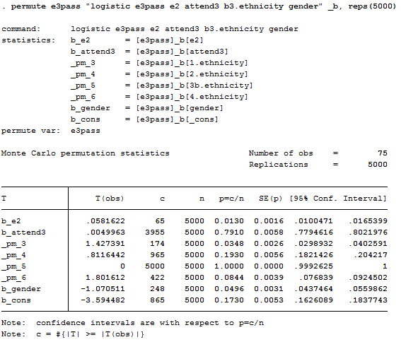
Let’s look first at some results for simple binary logistic regression predictions of the odds that an individual achieved a score of 70 or higher on the final exam. In Table 6.1, several models are presented that begin with individual actor attributes, then add predictors describing global and local network position effects, and finally add effects of network influence. Figure 6.14 shows the Stata syntax and output used to generate model 2. Figure 6.15 shows the Stata syntax and output used to test the significance of the coefficients in model 2 by Monte Carlo permutation. To run these analyses, we created a standard attribute data set (actors by attributes), and used Stata’s logistic regression command, followed by the post-estimation “estat” command to get information criteria measures for the models. Stata’s permute command was used to generate tests of significance for the model coefficients (with 5000 replications). Asian was used as the reference category for ethnic identity because it was the modal category. Odds ratios are shown in Table 6.1.
Table 6.1. Logistic Regression Models Predicting Passing the Final Exam
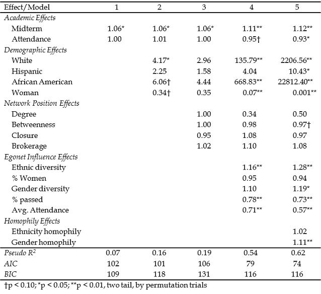
Figure 6.13. Stata Syntax and Output for Logistic Regression of Passing Final Exam (Model 2)
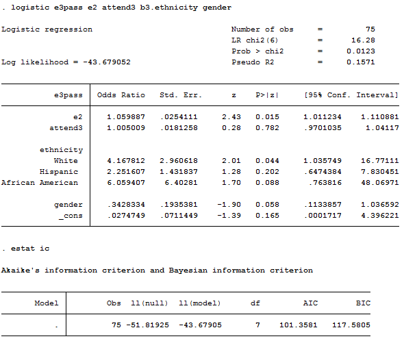
Figure 6.14. Stata Syntax and Output for Permutation Tests of Logistic Regression Parameters (Model 2)
In the first model, we predict passing the final exam based on whether the individual passed the mid-term, and their attendance at lecture between the mid-term and the final. The coefficients, which indicate how unit changes in the predictor multiply the odds of passing the exam, demonstrate that passing the mid-term exam has positive effects on passing the final exam. From the permutation trials, we find that effects of the size observed here occur in less than 5% of randomly permuted networks.
The second model adds the individual attributes of ethnicity and gender. Both ethnic identity and gender appear to affect the likelihood of passing the final exam for this social networks class.
The third model includes measures about the embedding of ego in the global and their local network (degree, centrality, ego-network closure, and brokerage within the ego-net). These measures were generated using the procedures shown in figures 6.1 through 6.4 above. The degree variable is the in degree of each actor, which can be found using either the “Indeg” variable from the “wave4_2011-cent” data set created in figures 6.1 and 6.2, or the “size” variable from the “wave4_2011-EgoNet” data set created in figures 6.3 and 6.4. These are identical measures. To measure centrality, we chose to use the global betweenness centrality variable (“Between”) from the “wave_2011-cent” data set. To measure ego-network closure, we reverse coded the reach efficiency (“ReachE”) variable from the “wave4_2011-EgoNet” data set because high values of ReachE indicate low levels of closure (this can be reverse coded by multiplying by negative one or subtracting from the max value). Finally, we used the brokerage variable (“Broker”) from the “wave4_2011-EgoNet” data set. None of these variables appear to be strong predictors of passing the final.
The fourth model adds social influence variables that describe the composition of each student’s ego network. Specifically, we were interested in ego’s in-neighborhood, or the direct ties that claim to know ego and therefore may influence ego’s behaviors and attitudes. The ethnic diversity variable used was from the “wave4_2011-EgoComposition-Ethnicity” data set created via the procedures shown in figures 6.5 and 6.6. We used Blau’s measure of heterogeneity (“Hetero”) multiplied by 100. The same procedure was run to generate variables describing the gender composition of the ego-networks. We multiplied the output variable called “p2,” which is the proportion of category two for the gender variable (woman), by 100 to generate a “percent woman” variable. This is the percentage of ego’s direct ties that are women. We also used Blau’s heterogeneity measure (“Hetero”) multiplied by 100 to create a gender diversity variable. In Chapter 5, we created a dichotomous variable that measured whether or not each student passed the final exam (where we’ve defined passing as achieving 70% or greater). Following the same procedure used to create the “percent woman” variable, we generated a “percent passed” variable which tells us the percent of ego’s direct ties that passed the final exam. Finally, using the same procedure outlined in figures 6.7 and 6.8, we generated a variable that examines the average attendance score (the UCINET output variable name is “Avg”) for the final third of the term (the time period most relevant to the final exam) for ego’s direct ties. Interestingly, diversity in the ethnic identities of students’ direct ties significantly improves their odds of passing, however, students who have friends with higher mid-term scores and better attendance are LESS likely to pass the final exam!
The final model tests the effects of homophily. That is, what are the effects on individuals of being in a personal network that is mostly of the same gender or same ethnicity as themselves? The creation of a measure of ethnicity homophily was demonstrated in Figures 6.9 and 6.10. This variable (“PctHomophilous”) saved in the data set “wave4_2011-EgoHomoMeas-Ethnicity” was used along with a gender homophily variable created in the same manner (both were multiplied by 100 to convert to percentages). We note a tendency (net of all the other factors) for students who have friends that are mostly the same gender as themselves to have improved chances of passing the final exam.
If we had measured the outcome as the interval-ratio variable of score on the final exam, we could use a different version of the GLM. Table 6.2 shows the results of a parallel analysis using a Gaussian distribution and identity link function (i.e. classical OLS linear regression), with permuted significance tests.
Table 6.2. OLS Linear Regression Models Predicting Final Exam Score
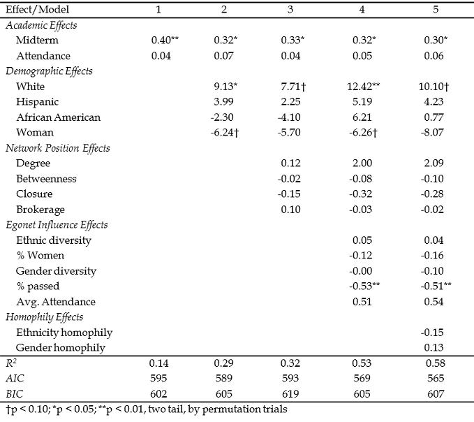
The analyses here are for illustration, and shouldn’t be taken very seriously (see the impossibly large odds ratios in the final column of Table 6.1). We are over-fitting the data with a model that is too complex. There are some substantial collinearities among the predictors. Most important, of course, there is no well-developed theory underlying the inclusion of terms. Do note, however, that the addition of measures of how ego is structurally embedded (models 3 and beyond), and social influence (model 4 and 5) do add considerably to our ability to predict the outcome, compared to a model based on individual attributes alone. However, from the BIC, we can see that this extra explanatory power comes at a cost.
Our approach to the effects of structural embedding and social influence are rather ad-hoc. In the next section, we will examine one more theoretically grounded approach to the study of social influence and diffusion processes based explicitly in exponential random graph theory (which we will discuss at some length in upcoming chapters).
The “autologistic actor attribute model” (AAAL) is a distinctive approach to examining processes of diffusion and influence that fits in the general “exponential random graphs” (ERG) framework that we’ll examine more closely in the next few chapters. An excellent recent presentation of the general approach to the AAAL is contained in Lusher, et. al (2013). A formal presentation of the model itself is given in Draganova and Robins (2013), and an illustration of its use to study network effects on employment status is provided in Draganova and Pattison (2013). The first of these works provides a very nice literature review that situates the AAAL within the ERG literature, and discusses precursors and competing approaches. Software for estimating AAAL (called iPNet) is available from http://www.melnet.org.au/pnet/, which is the home of the research group that has been a leading innovator in this field for many years.
At this writing, the AAAL model software supports the analysis of binary actor attributes (i.e. there are no versions for ordinal, multinomial, or interval-ratio attributes), and embedding in a symmetric binary network. The dependent variable is the presence or absence of the attribute for each ego, and ego’s attributes may be used to predict the log-odds of the presence of the attribute, just as we might if we were treating each ego as an independent observation.
The AAAL model, though, allows us to estimate a number of different kinds of social influence effects based on characteristics of ego’s one-step ego network. There are three general classes of social influence effects of this type: “network position” effects; “network-attribute” effects; and “covariate” effects.
“Network position effects” characterize some important aspects of the structure of each ego’s neighborhood, independent of attributes of the neighbors. These network position effects represent hypotheses about how the embedding of an ego in his/her local network may affect the probability that they have the attribute. Figure 6.15 (adapted from Daraganova and Robins 2013, table 9.1) graphically illustrates the types of network position effects that can be estimated with the AAAL. Note that the circles representing the alters directly or indirectly tied to ego (the shaded circle) are left unshaded which indicates that the presence or absence of the alters’ attribute is not important for these types of effects.
Figure 6.15. AAAL Network Position Effects
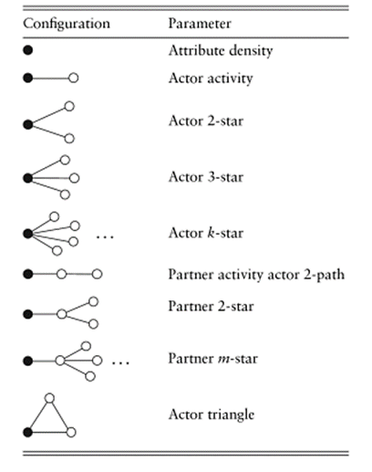
The first five effects form a hierarchy that models the majority of the variation in the degree-distribution of the graph. That is, these effects examine the hypothesis that egos that have fewer (or more) alters are less (or more) likely to exhibit the trait. Suppose that we were interested in predicting whether our students passed the final exam. We might think that students who had more acquaintances had more information, study partners, and social support, and would be more likely to pass the exam (regardless of their own attributes, or the attributes of their partners). The “actor activity” effect codes whether each ego has one (or more) alters. The “actor 2-star” effect codes whether an ego has two (or more) alters (controlling for whether they have any partners). The “actor 3-star” and “k-star” further differentiate actors who have still more alters from those who have none or fewer. Most degree distributions of actors are steeply exponential, so knowing whether actors have any alters or not, or knowing if they have more than one or two partners usually accounts for most of the variation in degree distributions.
The next three network position effects in figure 6.15 capture the idea that some actors are connected to others who are themselves well connected, while other egos may have equal numbers of partners, but those partners are less well connected. This is the notion of eigenvector or power/influence centrality. We might suppose, all else equal, that actors who are connected to well-connected others have easy access to large quantities of support, information, and influence. In our example, we might suppose that students who are well embedded in the “in-crowd” are in an advantaged position in preparing for the final exam.
The last network position effect in figure 6.15 is the “actor triangle.” Given that an ego has at least two alters, this effect asks: are these alters connected to one another? This gets at the idea of “clustering,” or “closure,” or lack of “structural holes” in ego networks. Actors who are tied to other actors who are also tied together (net of other structural effects) may have less efficient networks. Speculatively, we might suppose that students with neighborhoods characterized by “cliques” or closed structures may do more poorly on the examination because they have access to less unique information and perspective per social tie.
The network position effects of the AAAL are intended to capture the most important structural aspects of the ego-neighborhoods of each node (degree distribution, centrality, closure). They lead us to think about why some actors might be more likely to display an attribute based solely on how they are connected, regardless of the attributes of those to whom they are connected.
The next class of effects in the AAAL model, “network-attribute” effects, model specific forms of local autoregression. Figure 6.16 (again, adapted from Daraganova and Robins 2013) illustrates the effects available in iPNet. Notice now that certain alters directly or indirectly tied to ego are shaded, indicating that the presence or absence of those alters’ attribute is important for these types of effects.
Figure 6.16. AAAL Network-attribute Effects
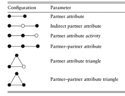
The most obvious, and often most important autoregressive effect is the “partner attribute” effect. It hypothesizes that the presence or absence of the dependent attribute for alter affects the probability that ego also has the attribute. The AAAL model also includes additional possible effects of the prevalence and location of the attribute in ego’s neighborhood on the likelihood that ego displays the attribute.
The “indirect partner attribute” hypothesizes that if ego’s direct-tie alter has an alter that has the attribute (regardless of whether ego’s direct-tie alter does), this indirect influence may affect ego’s outcome. The “partner attribute activity” effect hypothesizes that ego’s direct-tie alter may be more likely to lead ego to adopt the attribute if the direct-tie alter has alters (we are more influenced by others who are popular). This partner attribute activity effect may be even stronger to the extent that the direct-tie alter’s alters also display the attribute (“partner-partner attribute”). Again, as with network position effects, note that the network attribute effects are hierarchical – one must have effects from partners in order to also possibly have effects of partner’s partners. These effects suggest, for example, that the performance of the student’s friend’s friends on the exam may influence our focal student’s chances.
The last two effects in figure 6.16 combine the closure of ego’s neighborhood, and the prevalence of the attribute in that neighborhood. The “partner-attribute triangle” suggests that being in a closed neighborhood where anyone else has adopted the attribute may affect the likelihood of adopting. The “partner-partner attribute triangle” suggests that if ego is embedded in a clique where everyone else has the attribute, they are also likely to display it. If a student is in a clique where anyone passes the exam, or where everyone else passes the exam, they may themselves be more likely to pass the exam.
Finally, the AAAL model provides ways of modeling the effects of other attributes on the likelihood that ego displays a trait (“covariate effects”). Obviously, we might suppose that ego’s own attributes affect the likelihood that they display an attribute. For example, students who have done well on previous exams may be more likely to pass the final.
It also might be true that students who are tied to others with certain attributes may have different outcomes, regardless of their own attributes. In AAAL, these are called “partner-covariate” effects. For example, a student who is connected to others who did well on previous exams might be more likely to do well on the final.
Whether ego and alter are homophilous on other attributes may also by hypothesized to affect ego’s outcomes. In AAAL, such homophily effects are termed “same-partner-covariate” effects. If a man has a bias toward other men in his acquaintanceship network, he may be more likely to succeed (e.g. do well on a final examination) because of the sense of security and social support and trust that may be more common in homophilous ego-networks.
Taken together, the AAAL model provides a powerful tool-kit for examining social influence processes. It is a particularly interesting approach because it identifies and suggests hypotheses about effects on outcomes of the purely structural aspects of how actors are embedded in networks. It also includes a rich approach to understanding autoregressive effects, and the effects of other attributes of both ego and alter.
The iPNet software is relatively easy to use. It is available free for download, and is easy to install.
***iPNET example using student data coming soon***
So far, we’ve considered some ways to estimate the effects that the attributes of others have on an actor’s own attributes. In this section, we’ll look at ways in which we can control for special kinds of network influence effects that may act as nuisances in our models predicting attributes: network autoregressive and spatial error processes.
Network autoregression exists when ego’s score on an outcome attribute is determined (or at least predicted) by alter’s score on the same attribute. For example, we might hypothesize that a student’s score on the final exam is caused, or predicted, by his/her neighbor’s (in the ego-net) scores on the final exam. This kind of effect can be included in GLM (see section 6.3 above) and AAAL models. If ego’s neighbors do, in fact, exert social influence on ego, then it seems reasonable that ego may have outcomes that are more similar to his/her alters than to random others in the network. In GLM and AAAL models, we are trying to directly model the attributes of the alters that may affect ego’s outcome. If evidence of such effects exist, then there is autoregression in the network.
Network autoregressive models seek to control for these types of network influences, with the main goal of correctly estimating the effects of ego’s own attributes on ego’s outcomes. Unlike the GLM and AAAL approaches, network autoregressive models don’t try to directly examine the network influence processes, but simply remove these potentially confounding effects. Network autoregressive models provide a convenient way of controlling for network autoregressive influences of actors at greater network distances. If our interest is primarily in how ego’s attributes are associated with ego’s outcomes, we may well wish to simply control for, rather than directly model the effects of the alters’ outcome scores on ego’s outcome scores.
Network autocorrelated error exists when there are unmeasured local variables (errors, disturbances) that may affect the scores of both ego and ego’s alters on an outcome variable. Suppose that one student, while trying to prepare for the final examination, had a family crisis, and called on his/her friends in the class for support. We might suppose that ego’s score on the final exam would be lower than we would have expected on the basis of measured variables because of the “local disturbance” of having his/her study interrupted. But, we might expect that ego’s friend’s scores will also be negatively affected as they are deflected from preparing for the exam by supporting ego. In this case, both ego and his/her connected alters end up studying less for the final exam than we would have expected on the basis of their own attributes, resulting in a correlation of the error terms for ego, and the error terms for the alters.
Autoregressive and autocorrelated error models originate from geo-spatial analyses. In geo-spatial analysis, scores on some outcome (say, crime rates) are likely to be similar in places that are geographically close to one another. There are several processes that produce these spatial correlations. Because of exogenous processes (say the operation of the social class system of society), the attributes of actors who are spatially close are likely to be similar, producing similar outcomes (without any influence processes at all). The scores of spatially adjacent actors may also be similar because they are influencing one another. Criminals who practice their craft in one neighborhood are likely to also seek targets in adjacent spaces. But, there may be additional local disturbances that produce more similarity in crime rates in adjacent areas than we would otherwise expect. Perhaps we failed to measure and control for the level of policing, which is likely to be similar in adjacent neighborhoods. Having ignored this important variable will produce similar errors of prediction in adjacent neighborhoods.
To solve this problem, we simply apply the social network distance between the observations, and use the same approaches as geographical analysis, but with network distance, rather than spatial distance.
The network autoregressive process is also known as the “spatial lag model”. That is, the score on the outcome attribute of ego depends on the outcome attribute of ego’s alters, in addition to ego’s own attributes.
The network autocorrelated error model is also known as a model with “autoregressive disturbances”. In this model, the residuals or prediction errors of ego are correlated with the residuals or prediction errors of the alters.
It is possible, of course, to suppose that both lag and correlated error processes are operating.
To estimate models that correct for network auto regressive and/or autoregressive disturbances, the spreg package (Drukker, et al.) for Stata is rather easy to use. Pisani (2012) describes spreg as follows:
spreg estimates the parameters of a cross-sectional spatial-autoregressive model with spatial-autoregressive disturbances which is known as a SARAR model. A SARAR model includes a weighted average of the dependent variable, known as a spatial lag, as a right-hand-side variable and it allows the disturbance term to depend on a weighted average of the disturbances corresponding to other units. The weights may differ for each observation and are frequently inversely related to the distance from the current observation. These weights must be stored in a spatial-weighting matrix created by spmat. spreg estimates the parameters by either maximum likelihood (ML) or by generalized spatial two-stage least squares (GS2SLS).
Detailed documentation of the Stata packages needed for these types of models (also known as Cliff-Ord models) is available from Drukker, Peng, Prucha, and Raciborski (2013) and Drukker, Prucha, and Raciborski (2013). The packages are used to create spatial weighting matrices (spmat) and perform Cliff-Ord regressions (spreg).
Let’s again consider the problem of predicting our student’s scores on the final examination. We’ve already created the necessary input to do the analysis. In the section on GLM models (above), we created an attribute data set for our 75 students that includes individual attributes, measures of the location of each student in the global network (degree and betweenness centrality) and local neighborhood (closure and brokerage), and social influence (attributes of ego’s neighbors). Previously (in Chapter 5) we created a network distance weights matrix in order to test for autocorrelation. This is a student-by-student matrix of the reciprocal of geodesic distances. Of course, different definitions of distance could be used (for some ideas, see Chapter 5), and different distance matrices could be used for the autoregressive and error terms (we will use the same for both).
After locating and installing the sppack package (STATA: findit sppack), we locate our attribute file and distances file in a working directory (note the path and name). Estimation is a two-step process. First, we use the distance weights file we created last chapter (wave4_2011-geo.dta), and convert it to a form that can be used by the spatial regression package. We then load the attribute file (created for section 6.3 above), and perform regressions. Figure 6.17 gives the edited syntax of the STATA .do (i.e. batch) file that we used for this example (syntax for models 5 and 6 have been removed for brevity). Note, data files should be saved as .dta files prior to running. Also, make sure to specify the appropriate directory needed to find the data files.
Figure 6.17. STATA syntax used to create a distance matrix and perform several Cliff-Ord regressions
* Call in inverse
geodesic distance weights
use
"C:\SARAR\ wave4_2011-geo.dta", clear
* Create a
spatial-weighting matrix object
spmat
dta distwt var*
* Save the
spatial-weighting matrix object so that it can be called in when using
attribute data
spmat
save distwt using distwt.spmat, replace
* Open the
attribute data
use
"C:\SARAR\attributes", clear
* spreg wants the
id to be numeric, so gen a new id that goes from 1-75
gen
idnum = _n
*****
*
You would use the following line of syntax to call in the spmat objects
*
that were previously created with spmat.
*
spmat use distwt using distwt.spmat
*****
* Run the
regressions
* dlmat
uses spatial weights for network autoregression
* elmat
uses spatial weights for autocorrelated errors
* first model
includes only the autoregression based on inverse geodesic distance
spreg
ml e3, id(idnum) dlmat(distwt)
* get AIC and BIC
estat
ic
* second model
includes only the autocorrelated errors
spreg
ml e3, id(idnum) elmat(distwt)
estat
ic
* third model
includes both autoregression and autocorrelated errors
spreg
ml e3, id(idnum) dlmat(distwt)
elmat(distwt)
estat
ic
* fourth model
includes only covariates with no autoreg or autocorr
spreg
ml e3 e2 woman part btwcnt egosize pctwoman pctwhite, id(idnum)
estat
ic
*
seventh model includes covariates, autoregession, and autcorelated error
spreg
ml e3 e2 attend3 white hisp afam gender indeg between inv_reacheff
broker heteroeth pctwoman heterogen attendavg homoeth homogen,
id(idnum) dlmat(distwt) elmat(distwt)
estat
ic
Table 6.3 summarizes the results of seven different models predicting student’s scores on the final examination. The first models (1-3) include only the autoregressive and error correlation terms (separately and then together). The fourth model includes only covariates that describe attributes of ego, ego’s position in the network, and ego’s local neighborhood. The variables analyzed in section 6.3 were used again here. The spreg command does not support Stata’s “factor” variables so dummies were generated for ethnicity. We dropped the “percent passing the final” variable because it is, in effect, an autoregressive term. The final three models include the covariates and the autoregressive and autocorrelated error terms. The models are for instructional use only, and though they use real classroom data, they shouldn’t be taken seriously as testing a well specified theory of student performance.
Table 6.3. Cliff-Ord Regression Models Predicting Final Exam Score
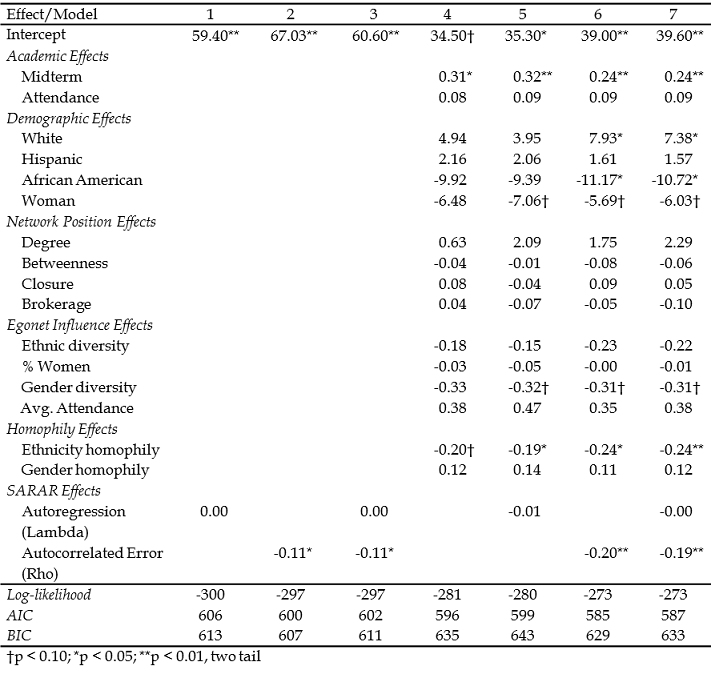
The significance of the coefficients taken with the goodness of fit statistics (deviance, AIC, BIC) suggest that including a network autocorrelated error term (Rho) is a useful addition to the covariates. However, accounting for autoregression (Lambda) does not appear to improve the model fit. Given the fit statistics, it appears that Model 6 might be the “best” model of the bunch.
We usually would anticipate that network autoregressive effects and network autocorrelated error effects would be positive quantities. That is, we would probably expect that being surrounded by others who do well on the exam would be associated with doing well oneself. This does not appear to be the case given the models that include Lambda. Similarly, we might expect that local disturbances (disturbances affecting an ego network, but not the whole network) would produce more similar outcomes among the members of the ego-network. However, the results above tell us just the opposite. These findings are consistent with the models in Tables 6.1 and 6.2 which find that being tied to others that pass the exam in one’s egonet causes students to do worse on the exam!
In this chapter we introduced models and techniques for capturing the ways in which network processes (e.g. social learning, social influence, diffusion) can influence nodal attributes. Using the student data introduced in Chapter 2, we provided examples demonstrating how to generate measures of network position, local influence (via egonets), and homophily in UCINET. We also discussed ways of generating spatial lags for response variables and spatial weights that can be used to model processes of autoregression and autocorrelation. We also briefly introduced Autologistic Actor Attribute Models, and finally, demonstrated how to control for autoregression effects and autocorrelated errors in Stata.
Burt, Ronald. 1992. Structural Holes: The Social Structure of Competition. Cambridge, MA: Harvard University Press.
Draganova, Galina and Pip Pattison. 2013. “Autologistic Actor Attribute Model Analysis of Unemployment: Dual Importance of Who You Know and Where You Live.” Pp. 237-247 in Dean Lusher, Johan Koskinen, and Garry Robins (Eds.), Exponential Random Graph Models for Social Networks: Theory, Methods, and Applications. Cambridge: Cambridge University Press.
Draganova, Galina and Garry Robins. 2013. “Autologistic Actor Attribute Models.” Pp. 102-114 in Dean Lusher, Johan Koskinen, and Garry Robins (Eds.), Exponential Random Graph Models for Social Networks: Theory, Methods, and Applications. Cambridge: Cambridge University Press.
Drukker, David M., Hua Peng, Ingmar R. Prucha, and Rafal Raciborski. 2013. “Creating and managing spatial-weighting matrices with the spmat command.” The Stata Journal, 13(2): 242–286.
Drukker, David M., Ingmar R. Prucha, and Rafal Raciborski. 2013. “Maximum likelihood and generalized spatial two-stage least-squares estimators for a spatial-autoregressive model with spatial-autoregressive disturbances.” The Stata Journal, 13(2): 221–241.
Gould, Roger V. and Roberto M. Fernandez. 1989. “Structures of mediation: A formal approach to brokerage in transaction networks.” Sociological Methodology, 19: 89-126.