Chapter 5. Association Between Attributes and Networks
In the previous two chapters we looked at studying association between two or more attributes of actors in a network (Chapter 3), and at studying association between two or more networks (Chapter 4). In this chapter, we’ll examine how to look at relationships between an attribute and a network.
What does it mean to examine the relationship between an attribute (node-level) variable, and a relational (dyadic-level) variable? This sounds a bit abstract. Let’s consider a couple of examples.
Citing the “homophily” principle (birds of a feather flock together), we might suppose that the women students from the classroom data (see Chapters 2-4) would be more likely to be acquainted with other women students than with men students in the class, and that men students were more likely to be acquainted with other men students. A student’s gender is a nodal, or attribute, or monadic variable. Whether acquaintanceships are woman-man, woman-woman, or man-man is a relational level variable. The variation being described is between pairs of nodes, not individuals. So, hypothesizing that there is gender homophily in relationships is actually making a prediction about the relationship between a nodal variable and a dyadic variable.
Citing the “social learning” principle (people are likely to be influenced by, and learn from those with whom they have social ties), we might suppose that students who are acquainted may have more similar grades. It may be that the students practice “network selection” in forming and breaking ties to increase similarity. Alternatively, it may be that students with social ties influence one another to become more similar. In either case, the correlation between students’ individual attributes (grades) is hypothesized to be a function of how far apart they are in the acquaintanceship network (which is a dyadic variable describing each pair of students).
In SNA, hypotheses that link the individual level and network level of analysis are common. Individual social actors may “select” which ties to make or break based on their own (or others) attributes. When social ties exist, individuals are influenced by the attributes of the others to whom they have ties. In SNA, nodal attributes may be independent variables that determine how an actor becomes embedded in the network (which dyads they are a part of). Nodal attributes may also be dependent variables that are affected by how the actor is embedded.
In later chapters, we will take a look at modeling these kinds of influence and selection processes that connect individuals and their networks. Often, our questions about the relation between an attribute and a network are quite simple and can be addressed with some rather simple tools. We’ll look first at a variety of approaches that are helpful when the attribute in question is categorical. For example, gender might be an independent attribute variable that affects the likelihood of acquaintanceship, or acquaintanceship might be an independent variable that affects test performance. Then, we’ll look at a rather different approach – borrowed from geo-statistics—that is helpful when the attribute being studied is interval-ratio.
Some of the most obvious, and also most important, questions about attributes and networks ask whether pre-existing nodal attributes determine how individuals are embedded in a network. Of course, the same kind of questions can be asked in reverse: to what extent does the way that an individual is embedded affect their individual attributes or behaviors.
There are several approaches that one can take. If the nodal attribute has two values (e.g. man or woman, passed the test or didn’t), a group-comparison approach can be used. If the nodal attribute has multiple values (e.g. ethnicity, which work group a person was in, which letter grade they earned on the final), a cross-tab approach can be applied. When the dyadic variable is either categorical or continuous, ANOVA density models or “block” models are a very interesting and useful approach.
5.2.1 Two Groups: Joint CountsLet’s suppose that our nodal variable is binary, and that our dyadic variable is also binary. We’ll consider two examples.
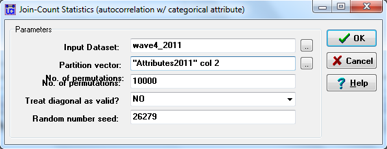
First, are there differences between men and women students in the gender of the others that they are acquainted with? Here, our nodal independent variable is whether a person identifies as a man or a woman. Our dyadic dependent variable is the count of the number of dyads that the individual is involved with that have a tie to a woman or a man. Here’s how we can test this hypothesis using UCIENET’s Tools>Testing Hypotheses>Mixed Dyadic/Nodal>Categorical Attribute>Joint Count. The dialog box used to set up the test is shown in figure 5.1.
Figure 5.1. UCINET Dialog for Testing Acquaintanceship Patterns by Gender

This looks a little mysterious. The “input dataset” is the location of the relational or dyadic variable of interest in the problem. Here, we have selected the matrix that describes whether each individual does, or does not claim to be acquainted with each other individual at the end of the course (wave 4). The “partition vector” is the column of the attribute data file that describes whether each individual is a man (coded 1) or a woman (coded 2). This happens to be the second column of our attributes data file.
To test whether there are differences between men and women in the likelihood that they form dyads with men or women, we will be using permutation tests, so the remaining parts of the dialog are defaults. Now, consider the output, shown in figure 5.2.
Figure 5.2. UCINET Output for Testing Acquaintanceship Patterns by Gender
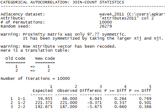
The procedure forms a cross-tabulation (not displayed). On one axis of the table is the attribute variable of whether the node is a man or a woman. On the other axis of the table is whether the other member of the dyad is a man or a woman. The output table “Expected” column shows the “joint count” of the number of man-man (1-1), man-woman (1-2) and woman-woman (2-2) dyads that we would expect to see if each respondent’s ties were distributed at random across all other persons (i.e. the number of each type of dyad we’d expect if the likelihood of a tie to a man or a woman was independent of ego’s gender). The “Observed” column shows how many such dyads were actually observed in the data.
In this example, we see that men students are more likely to affiliate with other men students than we would have expected under independence (they form 66 dyads with other men, rather than the 60 we would have expected if gender was irrelevant). Women students display a tendency to fewer ties with other women students than we would have expected (187 observed, versus 193 expected). However, differences this large in expected and observed counts happen rather frequently in joint-counts formed from randomly permuted data (that is, randomly assigning cases to dyadic ties with men or women). The p-level for man-man departure from independence is 0.264. For woman-woman dyads, the p-level is 0.366.
In a second example, let’s treat the individual attribute as dependent. First, let’s divide individuals into a partition (attribute) that measures whether they did, or did not, achieve a score of 70% or better on the final exam. This is an opportunity to demonstrate the power of UCINET’s Excel Matrix Editor. First open the editor by choosing Data>Data editors>Excel Matrix Editor or by clicking on the Excel icon in UCINET’s button bar across the top of the main window. Then choose Open>Open UCINET dataset and select the “Attributes_2011” file. In cell M1, create a new variable called “PassE3.” This variable will be coded “2” if the student received a score of 70 or better on E3 and “1” otherwise (UCINET’s Joint command sometimes has problems with “0”s for dichotomous attributes, so it’s best to avoid them). In cell M2, type “=if(J2>=70,2,1)” and hit Enter. Cell M2 now looks at cell J2 (which is student AD’s exam 3 score), checks whether it’s greater or equal to 70 (which it is) and codes either 2 or 1 for pass or fail respectively (it should read “2”). Now select M2 again, grab the small black square in the lower right corner and drag the cursor all the way down until you stop on cell M76. This now follows the same procedure for every student in the class and our new variable, PassE3, is ready to be used. Now save the data as a UCINET dataset and call it “Attributes_2011-PassE3,” to be used shortly.
For our independent variable, we’ll use a dyadic matrix that shows whether each pair of students were (coded “1”) or were not (coded “0”) in the same workgroup. We already did this in Chapter 2, where we created an actor-by-actor (i.e. 75 x 75) binary, symmetric matrix using Data>Partition to sets followed by Data>Affiliations (2-mode to 1-mode) and saved the dyadic data as “Same_work_groupRows”. Our research hypothesis is that students who are in the same workgroup are more likely to achieve similar outcomes on the final exam.
The dialog is the same as in figure 5.1, with “Same_work_groupRows” specified as the input dataset (dyadic variable), and “"Attributes2011-PassE3" col 12” (pass/fail on the exam) as the partition vector (nodal variable). The output is shown in figure 5.3.
Figure 5.3. UCINET Output Testing if Being in the Same Work Group Affects Passing the Final Exam
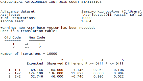
The “1-1” row shows dyads where both members failed the exam. There were 64 such dyads, slightly fewer than the number we would have expected under the null hypothesis of independence. Evidence against our theory. The “2-2” row is the count of dyads where both students passed the exam. There were significantly fewer (46) dyads than we would have expected under independence (53). And, the row “1-2” shows that there were 136 pairs where one member passed and the other failed. This happened more frequently than we would have expected under independence. It looks like we were wrong. If anything, there is a tendency for members of the same work groups to have different, rather than similar exam outcomes!
To reprise: in these examples we are examining whether there is an association between individual attributes and the frequency of involvement in dyads of particular kinds. In the first example, the individual’s attribute was the independent variable, gender, and the dyadic attribute was the gender mix of the dyads that they were embedded in. In the second example, the individual attribute of interest was dependent: whether the individuals involved in the dyad passed or did not pass the exam. The independent variable was the dyadic variable of being in the same work group or not.
5.2.2 Multiple Groups: A Contingency Table ApproachWe can expand the same kind of thinking to cases where the partition or attribute variable contains multiple categories. That is, we can look at the association between a dyadic or relational variable and a multi-valued attribute or nodal variable.
Let’s ask whether there is an association between which workgroups students were assigned to, and whether there are ties between them. Students were assigned to one of ten groups (a nodal variable), and were acquainted or not with each other student by the end of the term (a dyadic variable). We hypothesize that students are likely to have a higher density or probability of forming dyads with other members of their work group. Figure 5.4 shows the dialog for the UCINET “relational contingency table” tool (Tools>Testing Hypotheses>Mixed Dyadic/Nodal>Categorical Attribute>Relational Contingency Tables).
Figure 5.4. UCINET Dialog for Testing Acquaintanceship Differences among Work-Groups
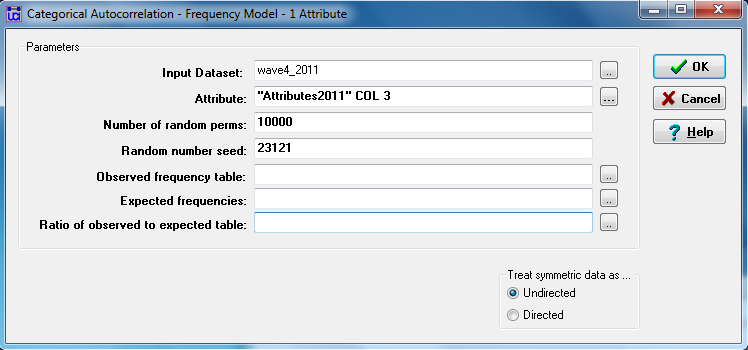
The “input dataset” is the square student-by-student dyadic acquaintanceship relation (we use wave 4, taken during the final exam). The “attribute” or categorical nodal variable is column 3 from the 2011 “Attributes” dataset, which contains the number of the work group to which each student was assigned. Again, there are controls for the permutation trials, and the option to save parts of the output as datasets for further processing. Figures 5.5.1, 5.5.2, and 5.5.3 show the full (somewhat lengthy) output.
Figure 5.5.1 UCINET Output for Testing Acquaintanceship Differences among Work-Groups (Part 1)
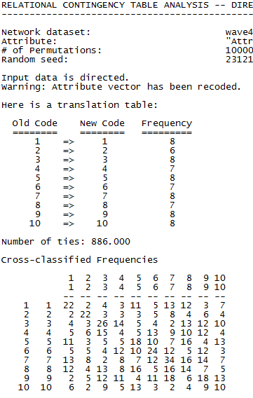
First we see the frequencies of the partition (work group number) variable. The groups varied in size between 6 and 8 students each. Next, we see the raw frequencies of the dyads formed by students in each group (row) with students in their own and other groups (column). For example, the students in group 1 claimed acquaintances 22 times with other members of their own group, only twice with a student from workgroup 2, eleven times with students in workgroup 5, and so on.
Note that the main diagonal looks pretty dense. That is, it looks like there is a tendency for students in each group to form dyads with other students in their same work-group. Also note that this tendency toward “homophily” isn’t the same across all work groups (note the diagonal value for group 4).
Figure 5.5.2 UCINET Output for Testing Acquaintanceship Differences among Work-Groups (Part 2)
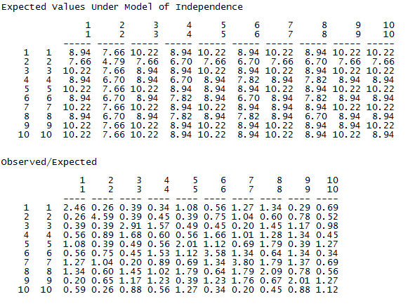
This part of the output doesn’t require much explanation. The expected counts under the null hypothesis of independence are displayed in the top panel and the ratio of observed to expected counts in the second panel. These are typical components of a chi-square based measure of association.
Figure 5.5.3 UCINET Output for Testing Acquaintanceship Differences among Work-Groups (Part 3)
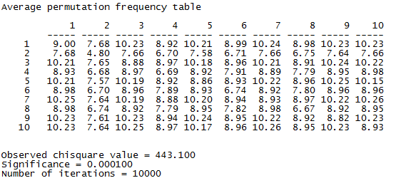
The penultimate bit of the output shows the expected counts under independence – that is, the mean counts observed across 10,000 runs with random assignment of students to workgroups. The differences between the observed and expected counts form a chi-square statistic (443.1). Using the sampling distribution from the permutation experiments, chi-squares this large are observed about one time in 10,000 for random trials.
So, we have strong evidence that there is an association between which work group a student is in (the nodal variable), and the probability that they are acquainted with a student sharing the same attribute (the dyadic variable). This result might be quite sufficient for many questions. But, we might want to go a bit further and explore the actual form of the association. ANOVA density models or “block” models are useful tools for this task.
5.2.3 Multiple Groups: ANOVA Density or “Block” ModelsUnder the homophily hypothesis, two students who have the same score on an attribute (in this case, being affiliated with a particular work group) may be more likely to know each other (have a dyadic relationship) than two students who do not have the same attribute. If this is the case, then the density of ties among the students in the same work group (regardless of which group it is) ought to be higher than the density of ties of students between students who are not in the same work group.
Imagine that we take our original student-by-student acquaintanceship matrix and re-arrange (permute) the rows and columns so that all the students in workgroup 1 are together, followed by workgroup 2, etc. We’ve “blocked” the matrix according to the “partition” of work-group. The blocked matrix is 10 by 10 groups.
Next, let’s count up all of the ties that exist in the blocks that fall along the main diagonal (that is, the block of group 1 with group 1, group 2 with group 2, etc.), and divide them by the number of possible ties. This is the mean, or probability that two actors who are in the same workgroup are acquainted.
Then, let’s count up all the ties between pairs of students who are not in the same work groups, and express this as proportion or mean of all possible ties that could have existed among these students.
We now have two groups (dyads in the same work group; dyads not in the same work group), and we can perform a test of differences of means, or one-way ANOVA. Figure 5.6 shows how to perform this particular two-group, one-way, ANOVA with UCINET’s Tools>Testing Hypotheses>Mixed Dyadic/Nodal>Categorical Attribute>ANOVA Density.
Figure 5.6 UCINET Dialog for Testing Acquaintanceship by Workgroup using a Constant Homophily Block Model
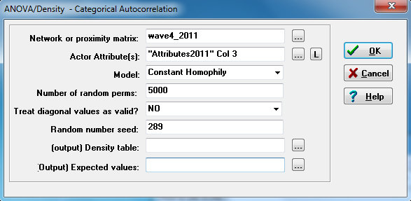
As always, there are controls for the permutation tests, and for saving parts of the output as UCINET files for further processing. We select our acquaintanceship dyadic data (it’s being treated here as the dependent variable), and the vector of work group affiliation from the attributes file (it happens to be the third column in that file).
The important part is the “Model,” where we’ve chosen “Constant Homophily.” The hypothesis that we have been discussing suggests that there is a difference in the likelihood of a tie between two actors in the same workgroup from the likelihood of a tie between two actors who are not in the same workgroup. Returning to our acquaintanceship matrix that has been blocked by workgroup, we are saying that the mean densities of all the blocks on the main diagonal (i.e. densities of ties to others in the same workgroup) are the same, and that the densities of all of the blocks not on the main diagonal (i.e. densities of ties to others outside of one’s group) are the same – and that these two densities differ. That is, there is a tendency toward homophily (the diagonal blocks differ from the non-diagonal blocks), and this tendency is constant across work groups (the density of ties within workgroup 1 is the same as the density of ties within workgroup 2, etc.). If we expected the tendency toward homophily to vary by work group, we could choose “Variable Homophily” instead. If we were interested in tendencies for out-group tie formation (vs. the in-group tendencies assumed in homophily assumptions), we would choose “Structural Blockmodel.” Figure 5.7 shows the output for our constant homophily model.
Figure 5.7 UCINET Output for Testing Acquaintanceship by Workgroup using a Constant Homophily Block Model
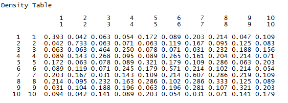
The first portion of the output shows the block densities actually present in our data. That is, it shows the mean density (or with a binary variable, the probability) of a tie between any two actors within a given block. For example, two students in work-group 1 have a 0.393 chance of having a tie, while the probability of a tie from a student in group 1 to group 3 is only 0.063. Just looking at the data, we see that the densities on the main diagonal (homophilic ties) are generally higher than those off of the main diagonal. We also should note that the densities of the blocks on the main diagonal are not very “constant” or similar to one another. Different work-groups have rather different degrees of homophily.
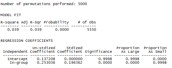
The next panels of the output describe how well the constant homophily block model does in explaining or predicting ties between pairs of actors. The answer is: not very well. Classifying dyads as being either within the same work group or not in the same workgroup explains about 4% of the variance in the probability that there is a dyadic tie. Note, however, that the permutation trials test very strongly suggests that workgroup homophily does have an effect (p < 0.0001).
The last part of the output shows, and tests, specific mean differences as regression coefficients (or effects in ANOVA language). We see that the mean probability of a tie between two students who are not in the same workgroup (the reference category or intercept) is 0.137. The probability of a tie between two students who are in the same work group is 0.253 higher, or 0.39. We see that this is a significant difference. Even though the variance explained is not high, being in the same work group more than doubles the probability of a dyadic tie between two students.
The constant homophily block model expresses a pretty strong hypothesis that suggests that there are no meaningful differences across workgroups in their tendency toward in-group tie formation. It also suggests that the bias against out-group acquaintances are the same, regardless of the out-group. An alternative model might propose that the bias against ties outside ones group are the same for all outsiders, but that groups differ in their tendency toward in-group ties. This hypothesis is selected by choosing the “variable homophily” block model in the dialog (figure 5.6). The output for this model is shown in figure 5.8.
Figure 5.8 UCINET Output for Testing Acquaintanceship by Workgroup using a Variable Homophily Block Model
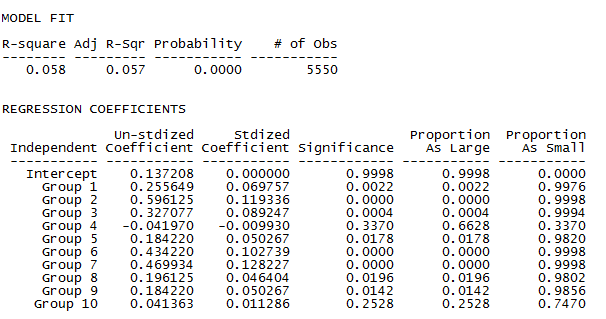
We see that the variable homophily model provides an improvement in fit (R-squared is 0.058, up from 0.039). The result is very unlikely to arise from random processes, but the model does not account for very much of the variation in who is acquainted with whom.
This improvement in fit has been bought at the expense of 9 additional parameters. Now, the tendency toward homophily in each of the 10 workgroups is allowed to differ from the intercept (which is the probability of a tie with an out-group student). The groups vary considerably in their tendency toward internal ties, as we see from the slopes describing how the density within each significantly differs from the intercept (group 4 and group 10 being exceptions).
The variable homophily block model allows for differences among groups in their preference for in-group ties. It treats all ties outside one’s own group as homogeneous. We can take the final step of relaxing this assumption with the “structural block model” option in the ANOVA density models dialog. Only a portion of the lengthy output is shown in figures 5.9.
Figure 5.9 UCINET Output for Testing Acquaintanceship by Workgroup using a Structural Block Model
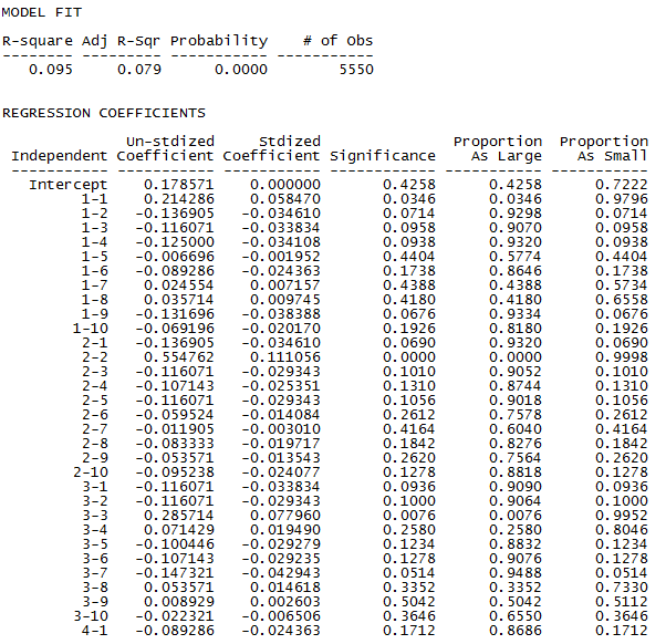
The structural block model allows each of the 10 by 10 blocks to vary in density. The variance explained by allowing variation in the external tie densities is relatively substantial (up to 9.5% from 5.8%). But, the gain is bought at the expense of 99 degrees of freedom. Every one of the 10x10 blocks is deviated from the last block (group 10 ties with group 10).
The ANOVA density, or “block” model allows fitting a variety of hypotheses about how a categorical attribute partitions (or blocks, or relates to) a relational (dyadic) variable. The relational variable can be either binary, as in our example, or continuous. For example, the relational variable might express the strength of ties in dyads, or it might express the network distance between two actors. So, block modeling can be used with categorical attributes and either categorical or continuous relational variables.
In looking at the relationship between an attribute and a network, when the attribute of interest is continuous, spatial autocorrelation methods can be used. These methods are borrowed from geographical analysis, and are adapted to use “social distance” between actors in a network, rather than spatial distances.
The type of question that we are addressing here is whether actors who are closer to one another in a network are likely to have the same score on an attribute. For example, we might ask whether students who know one another have similar exam scores. Questions like this one lie at the core of social influence theory, where it is hypothesized that the stronger the ties are between two actors, the more likely they are to converge in attitudes and behaviors as they model on and influence one another.
The core idea of network autocorrelation is that the correlation between the attributes of two members of a dyad covaries with the distance or strength of the tie between them. The basic method for assessing this is, logically, pretty simple. For each dyad, the individual nodal scores of both actors on some attribute are recorded (for example, the final exam scores of AD and AJ). Some measure of the strength of the tie or of the network distance between the two actors is generated (for example, say that the geodesic distance from AD to AJ is two steps of acquaintanceship, details below). The scores on the attribute of the two members of the dyad are then correlated across dyads, but weighted according to closeness or strength of the tie between them. The result is a distance-weighted correlation that tells us whether two actors who are close together are likely to have similar scores on the attribute (positive autocorrelation, most common) or are likely to have dissimilar scores on the attribute (negative autocorrelation), or if distance is irrelevant to the correlation between the scores of the members of dyads.
To examine autocorrelation, we need the attribute of interest for each actor. This is simply the attribute vector (e.g. test scores). We also need a measure of the distance between the two actors, so that we can “weight” the data. These weights are a dyadic variable describing the distance or strength of the tie between the members of the dyad.
In spatial autocorrelation applications (from which SNA appropriated these methods), the distance between two nodes (say locations on a map) is a fairly straightforward idea (actually, geo-spatial approaches to distance can be quite subtle, interesting, and complex). But, how do we measure “social distance?” There is no single best answer, but consider some possibilities.
One possible measure of dyadic distance for autocorrelation weighting is social similarity (such as distance in “Blau-space”; McPherson & Ranger-Moore, 1991). A dyadic variable could be created that measures similarity across a variety of attributes, or similarity in patterns of affiliation, for each pair of actors. Scaling, clustering, and index construction methods might then be used to calculate a “similarity” matrix for dyads.
Another, more concrete approach to creating distance weights is to see how far apart two actors are in a social network, directly. If AB names AJ as an acquaintance, the distance between them is 1 step. If AB names AJ and AJ names BL (and AB does not name BL), then the distance between AB and BL is 2 steps. Geodesic distance (the length of the shortest path from one actor to another) is a common approach and can be directly generated by UCINET (Network>Cohesion>Geodesic Distances).
Of course, the adjacency matrix can also be used directly. In this case, the distance between two actors in a network is either zero or one. Or, if the ties were measured on a continuous scale of strength, the matrix of tie strengths can be used directly.
For our example, we’ll define the distance between two students as the length of the geodesic path between them. But, since we would like a positive autocorrelation to mean that similarity increases with nearness (not distance), we will need to reverse the direction of the weights. We could simply subtract each distance from the maximum distance to measure closeness rather than distance. But, we are going to take the reciprocal of the geodesic distance instead. The reciprocal of the geodesic distance not only indexes “nearness,” but it also scales the data so that influence declines at an accelerated rate as distance increases (adjacent actors get a weight of 1/1 or 1.0; actors at a distance of two get a weight of 1/2 or 0.5, etc.).
Figure 5.10 shows the dialog for generating nearness (inverse distance) weights for our acquaintanceship data at the time of the final exam in UCINET by asking for geodesic distances (UCINET>Network>Cohesion>Geodesic Distances), rescaled by taking the reciprocal.
Figure 5.10 UCINET Dialog Used to Generate Inverse Geodesic Distances for Wave 4 Directed Acquaintanceship
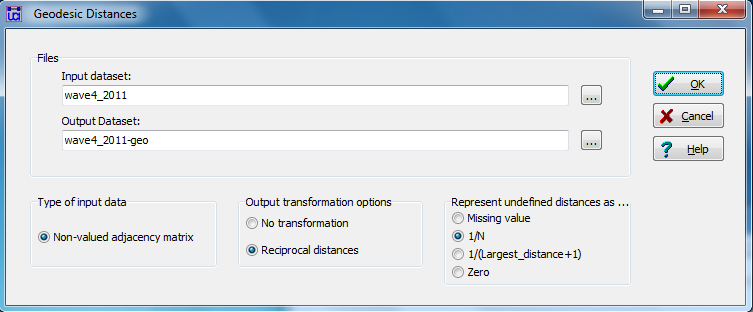
We can save the dyadic nearness variable that we’re creating as a new dataset and take the default name. Notice that we’ve marked the circle “1/N” in order to produce reciprocal distance values.
A portion of the nearness weights matrix is shown in Figure 5.11. We can also see from the figure that the most frequently occurring nearness weight is 0.5 which corresponds to a degree of 2.
Figure 5.11 UCINET Output for the Inverse Geodesic Distances of Wave 4 Directed Acquaintanceship
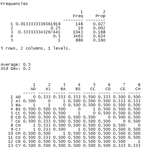
For network autocorrelation methods, a distance weighting matrix is needed. It is a dyadic variable that measures how similar, strong, or close the tie is between each pair of actors. As you can see, measuring the social distance between the two members of a dyad might be done in a wide variety of ways. And, as you can readily imagine, how one defines distance and creates a nearness weighting matrix can dramatically affect the results of an analysis. Our example is only one possible approach.
Once we have decided what attribute we want to test for network autocorrelation, and once we have created a distance or nearness weighting matrix, it is quite simple to generate some standard measures of network autocorrelation in UCINET (UCINET>Tools>Testing Hypotheses>Mixed Dyadic/Nodal>Continuous Attributes>Moran/Geary statistics). Figure 5.12 shows the dialog.
Figure 5.12 UCINET Dialog for Network Autocorrelation
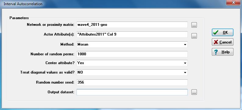
In the first box of the dialog, the nearness weights dyadic variable is identified. Note that any dyadic variable could be used – measures of social similarity, joint affiliation, as well as geographic or network distance. In the second box of the dialog the attribute that we want to examine for autocorrelation is identified. Here we identify column nine of the attribute dataset: student’s grades on the final exam (an interval/ratio variable). Distance (or nearness) weighted autocorrelations can, of course, be calculated for binary or ordinal-scale attributes, but the correlation measures were intended for continuous attributes.
5.3.1 Global Network AutocorrelationThere are quite a number of measures of spatial autocorrelation that have been developed, primarily by geo-scientists (Getis and Ord, 1992; Griffith, 1987). UCINET provides the two most commonly used: Moran and Geary indexes. The Moran index (and some others, as we will see below) summarizes the global pattern of autocorrelation over the entire network. That is, it looks across the whole network, seeking broad patterns. In our example using final exam grades, the Moran index is “looking” for big regions of the network that are occupied by mostly high scoring students and other big regions, or network neighborhoods, or communities that are composed mostly of low scoring students. The Moran index is somewhat less sensitive to an individual’s immediate neighborhoods.
In figures 5.13 and 5.14 the output of Tools>Testing Hypotheses>Mixed Dyadic/Nodal>Continuous Attributes>Moran Geary Statistics is shown (selecting the Moran statistic) using two different measures of nearness. In the first run (shown in figure 5.13), we use simple adjacency (A is acquainted with B, or not) as our measure of the network closeness or nearness weight. The “network or proximity matrix” used to generate the output in figure 5.13 is our wave 4 acquaintance data (“wave4_2011”). In the second run (figure 5.14), we use the reciprocal of the geodesic distance as our nearness weights (“wave4_2011-geo”). The dialog box shown in figure 5.12 generates the output shown in figure 5.14.
Figure 5.13 UCINET Output for Network Adjacency Autocorrelation of Final Exam Grades (Moran Index)
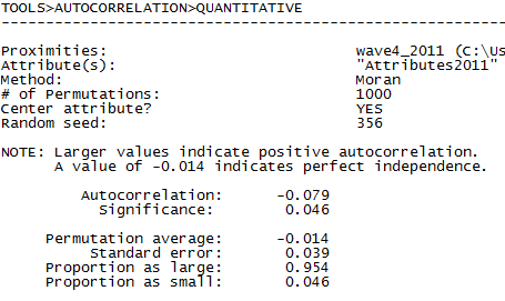
Figure 5.14 UCINET Output for Network Inverse Geodesic Distance Autocorrelation of Final Exam Grades (Moran Index)
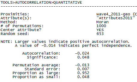
Interpreting the Moran statistic is a bit tricky in our case. Larger negative values of the Moran statistic indicate positive autocorrelation (here, a tendency for students with similar final exam scores to be adjacent or at shorter distances in the network) because we are using nearness weights rather than the typical use of distance. Significance tests are performed, as usual, using permutation (randomly shuffling the attribute scores).
When nearness is defined strictly as adjacency (Fig. 5.13), we see a modest positive autocorrelation (Moran statistic = -0.079) that is significant at the p = 0.05 level. When we apply inverse distance weights (Fig. 5.14), including indirect alters, the positive autocorrelation is weaker (-0.024).
In either case, we see a weak, but probably non-random, tendency for the network as a whole to display communities, regions, or neighborhoods occupied by students with similar grades on the final exam. There is some evidence that knowing one another and having similar grades are weakly associated.
5.3.2 Local Network AutocorrelationThe Geary statistic is constructed somewhat differently from the Moran, and places a greater emphasis on local patterns in the network. Rather than focusing on the network as a whole and looking for large regions of similar actors, it focuses on each actor’s local ties and then aggregates local autocorrelations into a global average. Figures 5.15 and 5.16 show the Geary autocorrelations of student’s grades where nearness is defined as adjacency (figure 5.15) or the reciprocal of geodesic distance (figure 5.16).
Figure 5.15 UCINET Output for Network Adjacency Autocorrelation of Final Exam Grades (Geary Index)
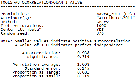
Figure 5.16 UCINET Output for Network Inverse Geodesic Distance Autocorrelation of Final Exam Grades (Geary Index)
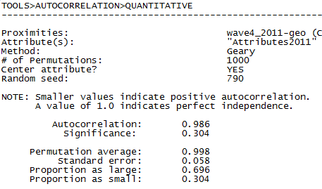
The Geary statistic is a somewhat odd metric. With Geary, more positive values indicate larger positive autocorrelations because we are using nearness matrices rather than the typical distance matrices used in geospatial analyses. However, the statistic ranges from zero, indicating perfect negative autocorrelation, to +2.0, indicating perfect positive autocorrelation. A value of +1.0 indicates no autocorrelation. Our values of 0.938 and 0.986 reported in our results, indicate a very slight negative autocorrelation, on the average, among the neighborhoods of individual students, but the effect is not significant in either case.
The values for the Geary statistics for both models of nearness are in the opposite direction from the Moran values. But, the Geary statistic does not reach statistical significance (at the p = 0.05 level) in either model. As with the Moran statistic, the magnitude of autocorrelation is stronger using simple adjacency, rather than inverse geodesic distances. This may not be surprising for many social influence processes (e.g. what our friend thinks of us is important, but what a friend of a friend thinks of us may not be relevant).
5.3.3 Network Autocorrelation with StataUCINET provides quick and easy calculation of the two most commonly used spatial autocorrelation measures, and good tools for constructing distance-weighting dyadic variables. Other software is available that can calculate additional measures of autocorrelation, and more importantly, use autocorrelation in predictive regression models. Maurizio Pisati (2001, 2012) has built a set of routines in Stata that are helpful for these tasks. Here, we’ll briefly illustrate how to use these tools for calculating measures of autocorrelation. In the next chapter, we will apply them to regression models that include network autocorrelation.
First, we need to locate and download the toolkit that Pisati has built by doing a findit in Stata. The components that are needed are spatwmat (which imports a distance weights matrix and calculates the needed eigenvectors), spatgsa (which calculates the Moran measure of global spatial autocorrelation), and spatlsa (which calculates local versions of the Moran measure for individual neighborhoods). The library “spatreg” (which performs spatial autoregression models) will be used in the next chapter. Stata help files come with the libraries, and can be viewed with the help command (help spatwmat for example) after the libraries are installed.
Second, we need to create Stata data files (i.e. “.dta” files) for our attribute (student grades), and social distance weights (we’ll use the reciprocal geodesic distances for our illustration). First, make sure that the rows and columns of the distance weights data are in the same sort order, and that the sort order agrees with that of the attributes dataset. Then, one can cut-and-paste, or use exports and imports to create two data sets in Stata. Figures 5.17 and 5.18 show partial screenshots of our two datasets.
Figure 5.17 Stata Data Editor Displaying Attributes Data Stored as a “.dta” File
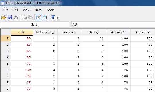
Figure 5.18 Stata Data Editor Displaying Distance Weights Matrix Stored as a “.dta” File
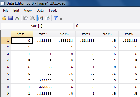
Note that the variable names (names of the nodes) are not included as a variable in the distance file, which has arbitrary variable names.
The third step of the process is to run spatwmat to generate the necessary formatted distances and store them in a temporary file in the working directory. Figure 5.19 shows how we did this step.
Figure 5.19 Stata Syntax for Running spatwmat Command
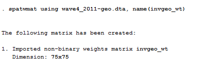
The Stata command tells the processor to run spatwmat using the distance weights Stata file we created (“wave4_2011-geo.dta”). After the comma (which delimits options in Stata), is the required option of name(), where you provide a name for the temporary weights file. We called ours “invgeo_wt.” Spatwmat reports that it created a non-binary weights matrix of 75x75.
Finally, we are ready to calculate measures of global autocorrelation for the variable “E3” which is the score on the final examination. Figure 5.20 shows how this is done. Note this must be done in the same working session where we create the temporary data file with the weights!
Figure 5.20 Stata Syntax and Output for Global Autocorrelation of Final Exam Using spatgsa
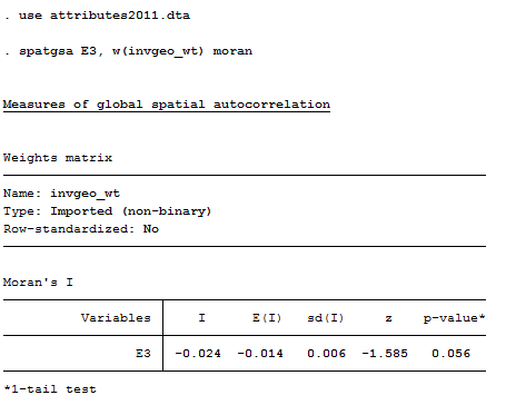
The Moran statistic is negative, indicating a positive global autocorrelation of student’s grades on the final exam. The value calculated in Stata (-0.024) is identical to the one calculated in UCINET to at least three decimal places (see Figure 5.14). The significance level reported by Stata, however, is slightly more conservative than the UCINET result. Minor differences are not unusual given the use of permutation trials.
Calculating the local version of the statistic can be done in the same working session with spatlsa, as shown in figure 5.21.
Figure 5.21 Stata Syntax and Output for Local Autocorrelation of Final Exam Using spatlsa
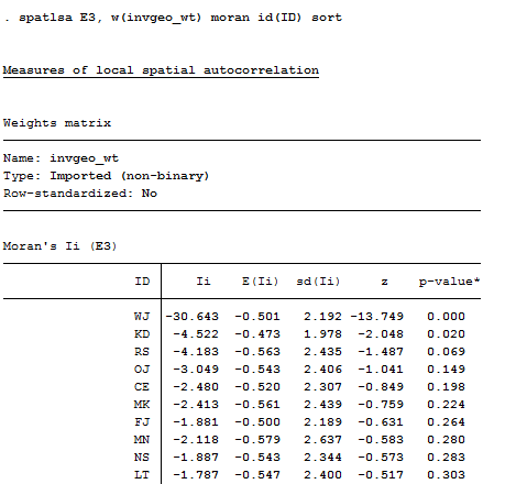
The syntax of the command is typical Stata: the procedure and variable list (multiple autocorrelations can be done in the same run) come first, followed by options after a comma. Here, the name of the weights matrix is supplied, the Moran statistic is specified (others are available, including Geary), the case name variable is identified to label the output, and a sort in order of decreasing positive autocorrelations is requested.
From the output, we see that the node WJ has an extremely strong positive autocorrelation of grades in his/her neighborhood, for example. The local autocorrelation of grades for each actor can be treated as an attribute of that actor describing something about the way in which they are embedded in the network. Indeed, one might think of the strength of the autocorrelation of grades as an indicator of the extent to which the actor has built ties with similar others, and/or been influenced by their neighbors. This is one way in which we might proceed to measure the degree of social influence on ego with regard to predicting ego’s grade on the final exam. That is, ego’s grade on the final exam might include a measure of how much ego is being influenced by his/her neighbor’s exam grades.
In this chapter we’ve had a look at some simple methods for examining the association between dyadic and nodal variables (i.e. social relations or networks and attributes). Analyses like the ones discussed here cross “levels of analysis” and involve both the attributes of the two individual nodes involved in a relationship, as well as information about the structure of the network in which they are embedded.
In analyses that include both individual attributes and network relations, our interest may focus on either as the dependent variable.
Sometimes we are primarily interested in how the ways in which actors are embedded in networks provide constraints and opportunities that shape or socially influence their own attitudes and behaviors (“social influence” models, Chapter 6). Sometimes we are interested in how individual attributes affect the processes by which social structures are selected or built by making and breaking connections (“network selection” models, Chapters 7 and 8). In many cases, both kinds of processes are occurring simultaneously as networks and the individuals that they connect co-evolve (Chapter 9).
In the remaining chapters, we’ll focus on modeling for these types of processes.
Getis, Arthur and J. K. Ord. 1992. “The analysis of spatial association by use of distance statistics.” Geographical Analysis, 24, 189-206.
Griffith, Daniel. 1987. “Spatial Autocorrelation: A Primer”. Washington, DC: Association of American Geographers Resource Publication.
McPherson, J. Miller and James R. Ranger-Moore. 1991. “Evolution on a Dancing Landscape: Organizations and Networks in Dynamic Blau Space.” Social Forces, 70(1): 19-42.
Pisati, Maurizio. 2001. “sg162: Tools for spatial data analysis.” Stata Technical Bulletin 60: 21-37. In Stata Technical Bulletin Reprints, vol. 10, 277-298. College Station, TX: Stata Press.
Pisati, Maurizio. 2012. “Spatial Data Analysis in Stata: An Overview.” 2012 Italian Stata Users Group meeting. Bologna, September 20-21, 2012. (slides available at: http://www.stata.com/meeting/italy12/abstracts/materials/it12_pisati.pdf)